Chapter 6 Clustering

6.1 Motivation

Clustering is an unsupervised learning technique that partitions a dataset into groups (clusters) based on the similarities between observations. In the context of scRNA-seq, cells in the same cluster will have similar expression profiles while cells in different clusters will be less similar. By assigning cells into clusters, we summarize our complex scRNA-seq data into discrete categories for easier human interpretation. The idea is to attribute some biological meaning to each cluster, typically based on its upregulated marker genes (Chapter 7). We can then treat the clusters as proxies for actual cell types/states in the rest of the analysis, which is more intuitive than describing population heterogeneity as some high-dimensional distribution.

6.2 Graph-based clustering

Popularized by its use in Seurat, graph-based clustering is a flexible and scalable technique for clustering large scRNA-seq datasets. We build a graph where each node is a cell that is connected to its nearest neighbors in the high-dimensional space. Edges are weighted based on the similarity between the cells involved, with higher weight given to cells that are more closely related. Clusters are then identified as “communities” of nodes that are more strongly interconnected in the graph, i.e., edges are concentrated between cells in the same cluster. To demonstrate, let’s use the PBMC dataset from 10X Genomics (Zheng et al. 2017):

# Loading in raw data from the 10X output files.
library(DropletTestFiles)
raw.path.10x <- getTestFile("tenx-2.1.0-pbmc4k/1.0.0/filtered.tar.gz")
dir.path.10x <- file.path(tempdir(), "pbmc4k")
untar(raw.path.10x, exdir=dir.path.10x)

library(DropletUtils)
fname.10x <- file.path(dir.path.10x, "filtered_gene_bc_matrices/GRCh38")
sce.10x <- read10xCounts(fname.10x, col.names=TRUE)

# Applying our default QC with outlier-based thresholds.
library(scrapper)
is.mito.10x <- grepl("^MT-", rowData(sce.10x)$Symbol)
sce.qc.10x <- quickRnaQc.se(sce.10x, subsets=list(MT=is.mito.10x)) 
sce.qc.10x <- sce.qc.10x[,sce.qc.10x$keep]

# Computing log-normalized expression values.
sce.norm.10x <- normalizeRnaCounts.se(sce.qc.10x, size.factors=sce.qc.10x$sum)

# We now choose the top HVGs.
sce.var.10x <- chooseRnaHvgs.se(sce.norm.10x)

# Running the PCA on the HVG submatrix.
sce.pca.10x <- runPca.se(sce.var.10x, features=rowData(sce.var.10x)$hvg)

# Running a t-SNE for visualization purposes.
sce.tsne.10x <- runTsne.se(sce.pca.10x)

We build a “shared nearest neighbor” (SNN) graph where the cells are the nodes. Each cell’s set of nearest neighbors is identified based on distances in the low-dimensional PC space, taking advantage of the compaction and denoising of the PCA (Chapter 4. Two cells are connected by an edge if they share any of their nearest neighbors, where the weight of the edge is defined from the number/rank of the shared neighbors (Xu and Su 2015). We then apply a community detection algorithm on the SNN graph - in this case, the “multi-level” algorithm, also known as Louvain clustering. Each node in the graph becomes a member of a community, giving us a cluster assignment for each cell (Figure 6.1).

sce.louvain.10x <- clusterGraph.se(sce.tsne.10x, method="multilevel")
table(sce.louvain.10x$clusters)

## 
##    1    2    3    4    5    6    7    8    9   10   11 
##  797  570 1007  127  382  503  224   36  183  118  200

library(scater)
plotReducedDim(sce.louvain.10x, "TSNE", colour_by="clusters")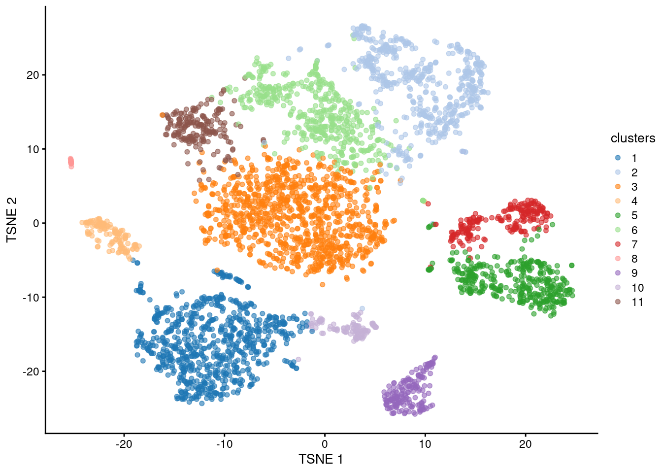

Figure 6.1: \(t\)-SNE plot of the 10X PBMC dataset, where each point represents a cell and is coloured according to the identity of the assigned cluster from graph-based clustering.

If we’re not satisfied with this clustering, we can fiddle with a large variety of parameters until we get what we want. (Also see discussion in Section 6.4.) This includes:

• The number of neighbors used in SNN graph construction (num.neighbors=). More neighbors increases the connectivity of the graph, resulting in broader clusters.
• The edge weighting scheme used in SNN graph construction. For example, we could mimic seurat’s behavior by using the Jaccard index to weight the edges.
• The resolution used by the community detection algorithm. Higher values will favor the creation of smaller, finer clusters.
• The community detection algorithm itself. For example, we could switch to the Leiden algorithm, which typically results in finer clusters.

sce.louvain20.10x <- clusterGraph.se(sce.tsne.10x, num.neighbors=20, method="multilevel")
table(sce.louvain20.10x$clusters)

## 
##    1    2    3    4    5    6    7    8    9   10 
##  808  508 1013  124  606  547   36  185  110  210

sce.jaccard.10x <- clusterGraph.se(sce.tsne.10x, more.build.args=list(weight.scheme="jaccard"))
table(sce.jaccard.10x$clusters)

## 
##    1    2    3    4    5    6    7    8    9   10   11   12 
##  742  537 1010  126  383  527  232   36  183  126  198   47

sce.lowres.10x <- clusterGraph.se(sce.tsne.10x, method="multilevel", resolution=0.1)
table(sce.lowres.10x$clusters)

## 
##    1    2    3    4    5    6 
## 1042  534 1746  606   36  183

sce.leiden.10x <- clusterGraph.se(sce.tsne.10x, method="leiden", more.cluster.args=list(leiden.objective="cpm"))
table(sce.leiden.10x$clusters)

## 
##   1   2   3   4   5   6   7   8   9  10  11  12  13  14  15  16  17  18  19  20 
## 130 126 149  46  57  74  16 171 151 151 102  72 115 125  91  88  36 152 161 140 
##  21  22  23  24  25  26  27  28  29  30  31  32  33  34  35  36  37  38  39  40 
##  23  45  85 123 129 190  71  56  80  81  95   8   3 111 116 133  34  47  75   9 
##  41  42  43  44  45  46  47  48  49  50  51  52  53  54  55  56  57  58  59  60 
##  45 104   4  48  85  13   1   5  71  29  35  13   4   3  15   1   1   1   1   1

Graph-based clustering has several appealing features that contribute to its popularity. It only requires a nearest neighbor search and is relatively efficient compared to, say, hierachical clustering methods that need a full distance matrix. Each cell is always connected to some neighbors in the graph, reducing the risk of generating many uninformative clusters consisting of one or two outlier cells. Community detection does not need a priori specification of the number of clusters, making it more robust for use across multiple datasets with different numbers of cell subpopulations. (Note that the number of clusters is still dependent on an arbitrary resolution parameter, so this shouldn’t be treated as an objective truth; but at least we avoid egregious cases of over- or underclustering that we might encounter with other methods like \(k\)-means.)

One drawback of graph-based methods is that, after graph construction, no information is retained about relationships beyond the neighboring cells¹⁹. This has some practical consequences in datasets that exhibit differences in cell density. More steps through the graph are required to traverse through a region of higher cell density. During community detection, this effect “inflates” the high-density regions such that any internal substructure is more likely to cause formation of subclusters. Thus, the resolution of the clustering becomes dependent on the density of cells, which can occasionally be misleading if it overstates the heterogeneity in the data.

On a practical note, the runAllNeighborSteps.se() function performs graph-based clustering alongside the \(t\)-SNE and UMAP. This is more efficient than calling each function separately, though results may be slightly different due to how the neighbor search results are shared across steps. We can sacrifice some speed for exact equality to the clusterGraph.se() results by setting collapse.search=FALSE.

sce.nn.10x <- runAllNeighborSteps.se(sce.pca.10x)
table(sce.nn.10x$clusters)

## 
##    1    2    3    4    5    6    7    8    9   10   11 
##  787  487 1022  135  383  563  223   36  182  129  200

reducedDimNames(sce.nn.10x)

## [1] "PCA"  "TSNE" "UMAP"

6.3 \(k\)-means clustering

\(k\)-means clustering is a classic technique for partitioning cells into a pre-specified number of clusters. Briefly, \(k\) cluster centroids are selected during initialization, each cell is assigned to its closest centroid, the centroids are then updated based on the means of its assigned cells, and this is repeated until convergence. This is simple, fast, and gives us exactly the desired number of clusters (Figure 6.2). Again, we use the per-cell PC scores for efficiency and denoising.

sce.kmeans.10x <- clusterKmeans.se(sce.tsne.10x, k=10)
table(sce.kmeans.10x$clusters)

## 
##    1    2    3    4    5    6    7    8    9   10 
##  484  177  226 1059  247  267  517  446  345  379

plotReducedDim(sce.kmeans.10x, "TSNE", colour_by="clusters")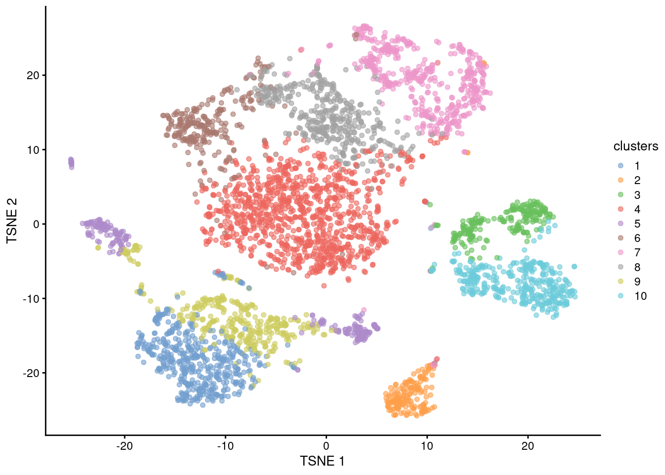

Figure 6.2: \(t\)-SNE plot of the 10X PBMC dataset, where each point represents a cell and is coloured according to the identity of the assigned cluster from \(k\)-means clustering.

If we’re not satisfied with the results, we can just tinker with the parameters. Most obviously, we could just increase \(k\) to obtain a greater number of smaller clusters. We could also alter the initialization and refinement strategies, though the effects of doing so are less clear. (By default, our initialization uses variance partitioning (Su and Dy 2007), which avoids the randomness of other approaches.)

sce.kmeans20.10x <- clusterKmeans.se(sce.tsne.10x, k=20)
table(sce.kmeans20.10x$clusters)

## 
##   1   2   3   4   5   6   7   8   9  10  11  12  13  14  15  16  17  18  19  20 
## 432 172 154 402 117 206 217 277  63 266 157 122 308 286  36 134 185 170  64 379

sce.kpp.10x <- clusterKmeans.se(sce.tsne.10x, k=10, more.kmeans.args=list(init.method="kmeans++"))
table(sce.kpp.10x$clusters)

## 
##    1    2    3    4    5    6    7    8    9   10 
##  444  225  267  335  704 1059  177  518   36  382

sce.lloyd.10x <- clusterKmeans.se(sce.tsne.10x, k=10, more.kmeans.args=list(refine.method="lloyd"))
table(sce.lloyd.10x$clusters)

## 
##    1    2    3    4    5    6    7    8    9   10 
##  483  177  226 1055  245  283  510  442  346  380

The major drawback of \(k\)-means clustering is that we need to specify \(k\) in advance. It is difficult to select a default value that works well for a variety of datasets. If \(k\) is larger than the number of distinct subpopulations, we will overcluster, i.e., split subpopulations into smaller clusters; but if \(k\) is smaller than the number of subpopulations, we will undercluster, i.e., group multiple subpopulations into a single cluster. We might consider some methods to automatically determine a “suitable” value for \(k\), e.g., by maximizing the gap statistic (Tibshirani, Walther, and Hastie 2001). This can be computationally intensive as it involves repeated clusterings at a variety of possible \(k\).

# Gap statistic involves the random generation of a simulated dataset,
# so we need to set the seed to get a reproducible result.
set.seed(999)

library(cluster)
gap.10x <- clusGap(
    reducedDim(sce.tsne.10x, "PCA"),
    FUNcluster=function(x, k) {
        # clusterKmeans() is the low-level function used by clusterKmeans.se().
        # We transpose the input as lusterKmeans expects cells in the columns.
        list(cluster=as.integer(clusterKmeans(t(x), k)$clusters))
    },
    K.max=50,
    B=5,
    verbose=FALSE
)

# Choosing the number of clusters that maximizes the gap statistic.
maxSE(f = gap.10x$Tab[,"gap"], SE.f = gap.10x$Tab[,"SE.sim"])

## [1] 26

In practice, we mostly use \(k\)-means clustering for vector quantization. Instead of attempting to interpret the clusters, we treat each centroid as a “pseudo-cell” that represents all of its assigned cells. These representatives are used as the input data of computationally intensive procedures, which is more efficient than operating on the per-cell data. We usually set \(k\) to a large value such as the square root of the number of cells. This yields a set of fine-grained clusters that approximates the underlying distribution of cells in downstream steps, e.g., hierarchical clustering (Figure 6.3). A similar approach is used in SingleR to compact large references prior to cell type annotation.

sce.vq.10x <- clusterKmeans.se(sce.tsne.10x, k=sqrt(ncol(sce.tsne.10x)), meta.name="kmeans")
table(sce.vq.10x$clusters)

## 
##   1   2   3   4   5   6   7   8   9  10  11  12  13  14  15  16  17  18  19  20 
##  69  71  68  85  83  43  65  51  38  54  63  56  81 143  11  56  64  51  79 112 
##  21  22  23  24  25  26  27  28  29  30  31  32  33  34  35  36  37  38  39  40 
##  15  29  15  74  11  93  10  39 176  44  53   2  86  65 128 118  30  43   7 104 
##  41  42  43  44  45  46  47  48  49  50  51  52  53  54  55  56  57  58  59  60 
##  19  69  41  45 129  66  31 107  16  50 142 116  89   1  57  58 117 119  59  89 
##  61  62  63  64 
##   2  66  72 102

vq.centers.10x <- metadata(sce.vq.10x)$kmeans$centers
dim(vq.centers.10x)

## [1] 25 64

# Using centroids for something expensive, e.g., hierarchical clustering. This
# involves creating a distance matrix that would be too large if we did it for
# each pair of cells; so instead we do it between pairs of k-means centroids.
dist.vq.10x <- dist(t(vq.centers.10x))
hclust.vq.10x <- hclust(dist.vq.10x, method="ward.D2")
plot(hclust.vq.10x, xlab="", sub="")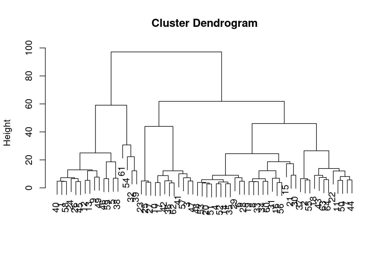

Figure 6.3: Dendrogram of the \(k\)-means cluster centroids from the PBMC dataset. Each leaf represents a centroid from \(k\)-means clustering.

# Cutting the dendrogram at a dynamic height to cluster our centroids. 
library(dynamicTreeCut)
cutree.vq.10x <- cutreeDynamic(
    hclust.vq.10x,
    distM=as.matrix(dist.vq.10x),
    minClusterSize=1,
    verbose=0
)
table(cutree.vq.10x)

## cutree.vq.10x
##  1  2  3  4  5  6  7  8 
## 14 11 11  9  9  4  3  3

# Now extrapolating to all cells assigned to each k-means cluster.
hclust.full.10x <- cutree.vq.10x[sce.vq.10x$clusters]
table(hclust.full.10x)

## hclust.full.10x
##    1    2    3    4    5    6    7    8 
## 1030 1180  607  606  518   12   36  158

6.4 Choosing the clustering parameters

What is the “right” number of clusters? Which clustering algorithm is “correct”? These thoughts have haunted us ever since we did our first scRNA-seq analysis²⁰. But with a decade of experience under our belt, our advice is to not worry too much about an “optimal” clustering. Just proceed with the rest of the analysis and attempt to assign biological meaning to each cluster (Chapter 7). If the clusters represent our cell types/states of interest, great; if not, we can always come back here and fiddle with the parameters.

It is helpful to realize that clustering, like a microscope, is simply a tool to explore the data. We can zoom in and out by changing the resolution-related clustering parameters, and we can experiment with different clustering algorithms to obtain alternative perspectives. Perhaps we just want to resolve the major cell types, in which case a lower resolution would be appropriate; or maybe we want to distinguish finer subtypes or cell states (e.g., metabolic activity, stress), which would require higher resolution. The best clustering really depends on the scientific aims, which are difficult to translate into an a priori choice of parameters or algorithms. So, we can just try again if we don’t get what we want on the first pass²¹.

For what it’s worth, there exist many more clustering algorithms that we have not discussed here. Off the top of our head, we could suggest hierarchical clustering, a classic technique that builds a dendrogram to summarize relationships between clusters; density-based clustering, which adapts to unusual cluster shapes and can ignore outlier points; and affinity propagation, which identifies exemplars based on similarities between points. All of these methods have been applied successfully to scRNA-seq data and might be worth considering if graph-based clustering isn’t satisfactory. For larger datasets, any scalability issues for these methods can be overcome by clustering on \(k\)-means centroids instead (Section 6.3).

6.5 Clustering diagnostics

If we really need some “objective” metric of cluster quality²², we can evaluate the stability of each cluster using bootstrap replicates. Ideally, the clustering should be stable to perturbations to the input data (Von Luxburg 2010), which increases the likelihood that they can be reproduced in an independent study. To quantify stability, we create a “bootstrap replicate” dataset by sampling cells with replacement from the original dataset. The same clustering procedure is applied to this replicate to determine if the clusters from the original dataset can be reproduced. In Figure 6.4, a diagonal entry near 1 indicates that the corresponding cluster is not split apart in the bootstrap replicates, while an off-diagonal entry near 1 indicates that the corresponding pair of clusters are always separated. Unstable clusters or unstable separation between pairs of clusters warrant some caution during interpretation.

# Bootstrapping involves random sampling so we need to set
# the seed to get a reproducible result.
set.seed(888)

library(bluster)
bootstrap.10x <- bootstrapStability(
    reducedDim(sce.louvain.10x, "PCA"),
    FUN=function(x) {
        # i.e., our clustering procedure. These are the low-level functions
        # that are called by clusterGraph.se(). Note that we transpose the
        # input as buildSnnGraph expects the cells to be in the columns. 
        g <- buildSnnGraph(t(x))
        clusterGraph(g, method="multilevel")$membership
    },
    clusters=sce.louvain.10x$clusters,
    adjusted=FALSE
)

library(pheatmap)
pheatmap(
    bootstrap.10x,
    cluster_row=FALSE,
    cluster_col=FALSE,
    color=viridis::magma(100),
    breaks=seq(0, 1, length.out=101)
)

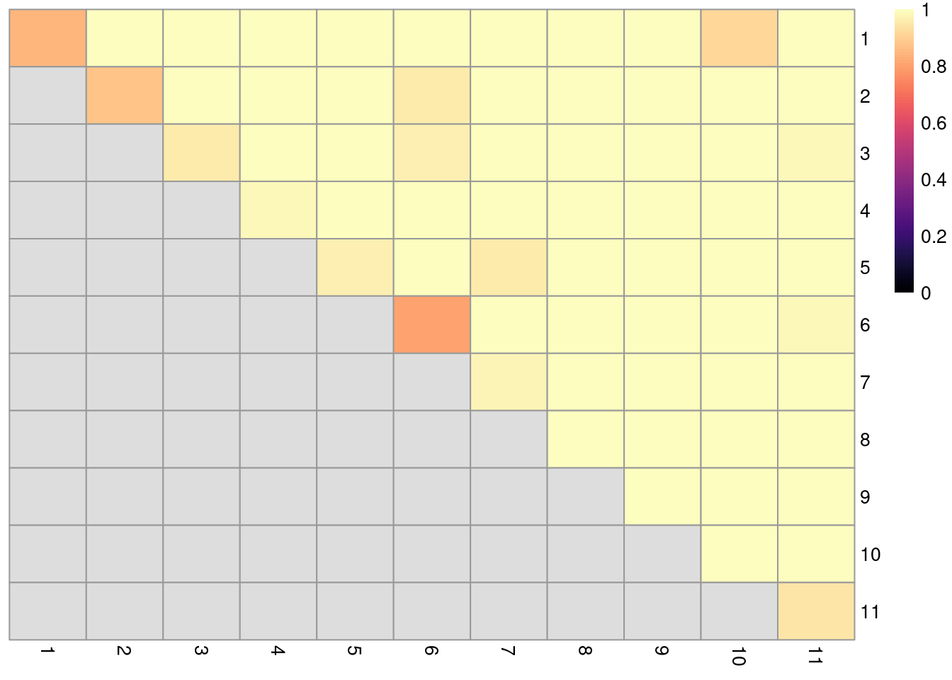
Figure 6.4: Heatmap of probabilities of co-clustering from bootstrapping of graph-based clustering in the PBMC dataset. Each row and column represents an original cluster and each entry is colored according to the probability that two cells from their respective row/column clusters are clustered together (diagonal) or separated (off-diagonal) in the bootstrap replicates.

If even more clustering diagnostics are required, we can choose from a variety of measures of cluster “quality” in the bluster package:

• The silhouette width, as implemented in the approxSilhouette() function. For each cell, we compute the average distance to all cells in the same cluster. We also find the minimum of the average distances to all cells in any other cluster. The silhouette width for each cell is defined as the difference between these two values divided by their maximum. Cells with large positive silhouette widths are closer to other cells in the same cluster than to cells in the nearest other cluster. Thus, clusters with large positive silhouette widths are well-separated from other clusters.
• The clustering purity, as implemented in the clusterPurity() function. The purity is defined for each cell as the proportion of neighboring cells that are assigned to the same cluster, after some weighting to adjust for differences in the number of cells between clusters. This quantifies the degree to which cells from multiple clusters intermingle in expression space. Well-separated clusters should exhibit little intermingling and thus high purity values for all member cells.
• The root mean-squared deviation (RMSD), as implemented in the clusterRSMD() function. This is root of the mean of the squared differences from the cluster centroid across across all cells in the cluster. It is closely related to the within-cluster sum of squares (WCSS) and is a natural diagnostic for \(k\)-means clustering. A large RMSD suggests that a cluster has some internal structure and should be prioritized for further subclustering.
• The modularity scores of the communities in the graph, as implemented in the pairwiseModularity() function. For each community,tThis is defined as the difference between the observed and expected number of edges between cells in that community. The expected number of edges is computed from a null model where edges are randomly distributed among cells. Communities with high modularity scores are mostly disconnected from other communities in the graph.

In general, we find these diagnostics to be more helpful for understanding the properties of each cluster than to identify “good” or “bad” clusters. For example, a low average silhouette width indicates that the cluster is weakly separated from its nearest neighboring clusters. This is not necessarily a bad thing if we’re looking at subtypes or states that exhibit relatively subtle changes in expression²³. One might be tempted to objectively define a “best” clustering by adjusting the clustering parameters to optimize one of these metrics, e.g., maximum silhouette width. While there’s nothing wrong with this approach, it may not yield clusters that correspond to our cell types/states of interest. Anecdotally, we have observed that these optimal clusterings only separate broad cell types as any attempt to define weakly-separated clusters will be penalized.

6.6 Subclustering

On occasion, we may want to investigate internal structure within a particular cluster, e.g., to find fine-grained cell subtypes. We could just increase the resolution of our clustering algorithm but (i) this is not guaranteed to split our cluster of interest and (ii) it could alter the distribution of cells in other clusters that we did not want to change. In such cases, a simple alternative is to repeat the feature selection and clustering within the cluster of interest. This selects HVGs and PCs that are more relevant to the cluster’s internal variation, improving resolution by avoiding noise from unnecessary features. The absence of distinct subpopulations also encourages clustering methods to separate cells according to more modest intra-cluster heterogeneity. Let’s demonstrate on cluster 2 of our PBMC dataset:

chosen.cluster <- "2"
sce.sub.10x <- sce.louvain.10x[,sce.louvain.10x$clusters == chosen.cluster]
dim(sce.sub.10x)

## [1] 33694   570

sce.subvar.10x <- chooseRnaHvgs.se(sce.sub.10x)
sce.subpca.10x <- runPca.se(sce.subvar.10x, features=rowData(sce.subvar.10x)$hvg)
sce.subtsne.10x <- runTsne.se(sce.subpca.10x)

We perform a new round of clustering on all of the cells in this subset of the data (Figure 6.5). This effectively increases our resolution of cluster 2 by breaking it into further subclusters. Importantly, we can increase resolution without changing the parameters of the parent clustering, which is convenient if we’re already satisfied with those clusters.

# We don't necessarily have to use the same parameters that we used to cluster
# the full dataset, but there's no reason to change either, so whatever.
sce.subgraph.10x <- clusterGraph.se(sce.subtsne.10x)
table(sce.subgraph.10x$clusters)

## 
##   1   2   3   4   5 
## 155 145  34 146  90

plotReducedDim(sce.subgraph.10x, "TSNE", colour_by="clusters")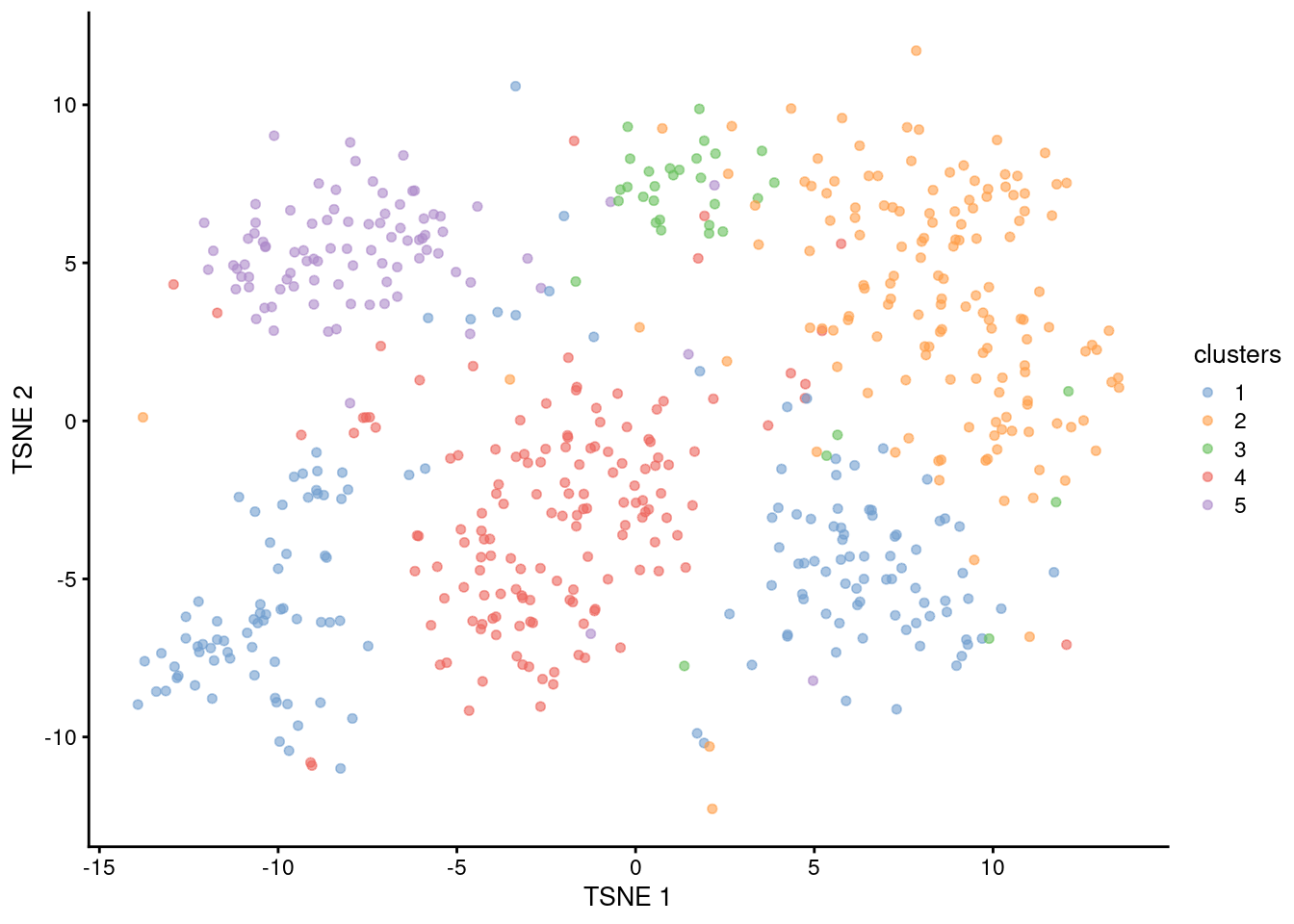

Figure 6.5: \(t\)-SNE plot of cells in cluster 2 of the 10X PBMC dataset, where each point represents a cell and is coloured according to the identity of the assigned subcluster from graph-based clustering.

Subclustering can simplify the interpretation of the subclusters, as these only need to be considered in the context of the parent cluster’s biological identity. For example, if we knew that the parent cluster contained T cells, we could treat all of the subclusters as T cell subtypes. However, this requires some care if there is any uncertainty in the identification for the parent cluster. If the underlying cell types/states span cluster boundaries, conditioning on the putative identity of the parent cluster may be premature, e.g., a subcluster actually represents contamination from a cell type in a neighboring parent cluster.

6.7 Session information

sessionInfo()

## R Under development (unstable) (2025-12-24 r89227)
## Platform: x86_64-pc-linux-gnu
## Running under: Ubuntu 22.04.5 LTS
## 
## Matrix products: default
## BLAS:   /home/luna/Software/R/trunk/lib/libRblas.so 
## LAPACK: /home/luna/Software/R/trunk/lib/libRlapack.so;  LAPACK version 3.12.1
## 
## locale:
##  [1] LC_CTYPE=en_US.UTF-8       LC_NUMERIC=C              
##  [3] LC_TIME=en_US.UTF-8        LC_COLLATE=en_US.UTF-8    
##  [5] LC_MONETARY=en_US.UTF-8    LC_MESSAGES=en_US.UTF-8   
##  [7] LC_PAPER=en_US.UTF-8       LC_NAME=C                 
##  [9] LC_ADDRESS=C               LC_TELEPHONE=C            
## [11] LC_MEASUREMENT=en_US.UTF-8 LC_IDENTIFICATION=C       
## 
## time zone: Australia/Sydney
## tzcode source: system (glibc)
## 
## attached base packages:
## [1] stats4    stats     graphics  grDevices utils     datasets  methods  
## [8] base     
## 
## other attached packages:
##  [1] pheatmap_1.0.13             bluster_1.21.0             
##  [3] dynamicTreeCut_1.63-1       cluster_2.1.8.1            
##  [5] scater_1.39.1               ggplot2_4.0.1              
##  [7] scuttle_1.21.0              scrapper_1.5.10            
##  [9] DropletUtils_1.31.0         SingleCellExperiment_1.33.0
## [11] SummarizedExperiment_1.41.0 Biobase_2.71.0             
## [13] GenomicRanges_1.63.1        Seqinfo_1.1.0              
## [15] IRanges_2.45.0              S4Vectors_0.49.0           
## [17] BiocGenerics_0.57.0         generics_0.1.4             
## [19] MatrixGenerics_1.23.0       matrixStats_1.5.0          
## [21] DropletTestFiles_1.21.0     BiocStyle_2.39.0           
## 
## loaded via a namespace (and not attached):
##   [1] DBI_1.2.3                 gridExtra_2.3            
##   [3] httr2_1.2.2               rlang_1.1.7              
##   [5] magrittr_2.0.4            otel_0.2.0               
##   [7] compiler_4.6.0            RSQLite_2.4.5            
##   [9] DelayedMatrixStats_1.33.0 png_0.1-8                
##  [11] vctrs_0.6.5               pkgconfig_2.0.3          
##  [13] crayon_1.5.3              fastmap_1.2.0            
##  [15] dbplyr_2.5.1              XVector_0.51.0           
##  [17] labeling_0.4.3            rmarkdown_2.30           
##  [19] ggbeeswarm_0.7.3          purrr_1.2.1              
##  [21] bit_4.6.0                 xfun_0.55                
##  [23] cachem_1.1.0              beachmat_2.27.1          
##  [25] jsonlite_2.0.0            blob_1.2.4               
##  [27] rhdf5filters_1.23.3       DelayedArray_0.37.0      
##  [29] Rhdf5lib_1.33.0           BiocParallel_1.45.0      
##  [31] irlba_2.3.5.1             parallel_4.6.0           
##  [33] R6_2.6.1                  bslib_0.9.0              
##  [35] RColorBrewer_1.1-3        limma_3.67.0             
##  [37] jquerylib_0.1.4           Rcpp_1.1.1               
##  [39] bookdown_0.46             knitr_1.51               
##  [41] R.utils_2.13.0            igraph_2.2.1             
##  [43] Matrix_1.7-4              tidyselect_1.2.1         
##  [45] viridis_0.6.5             dichromat_2.0-0.1        
##  [47] abind_1.4-8               yaml_2.3.12              
##  [49] codetools_0.2-20          curl_7.0.0               
##  [51] lattice_0.22-7            tibble_3.3.0             
##  [53] S7_0.2.1                  withr_3.0.2              
##  [55] KEGGREST_1.51.1           evaluate_1.0.5           
##  [57] BiocFileCache_3.1.0       ExperimentHub_3.1.0      
##  [59] Biostrings_2.79.4         pillar_1.11.1            
##  [61] BiocManager_1.30.27       filelock_1.0.3           
##  [63] BiocVersion_3.23.1        sparseMatrixStats_1.23.0 
##  [65] scales_1.4.0              glue_1.8.0               
##  [67] tools_4.6.0               AnnotationHub_4.1.0      
##  [69] BiocNeighbors_2.5.0       ScaledMatrix_1.19.0      
##  [71] locfit_1.5-9.12           cowplot_1.2.0            
##  [73] rhdf5_2.55.12             grid_4.6.0               
##  [75] AnnotationDbi_1.73.0      edgeR_4.9.2              
##  [77] beeswarm_0.4.0            BiocSingular_1.27.1      
##  [79] HDF5Array_1.39.0          vipor_0.4.7              
##  [81] rsvd_1.0.5                cli_3.6.5                
##  [83] rappdirs_0.3.3            viridisLite_0.4.2        
##  [85] S4Arrays_1.11.1           dplyr_1.1.4              
##  [87] gtable_0.3.6              R.methodsS3_1.8.2        
##  [89] sass_0.4.10               digest_0.6.39            
##  [91] ggrepel_0.9.6             SparseArray_1.11.10      
##  [93] dqrng_0.4.1               farver_2.1.2             
##  [95] memoise_2.0.1             htmltools_0.5.9          
##  [97] R.oo_1.27.1               lifecycle_1.0.5          
##  [99] h5mread_1.3.1             httr_1.4.7               
## [101] statmod_1.5.1             bit64_4.6.0-1

References

Su, T., and J. G. Dy. 2007. “In search of deterministic methods for initializing K-means and Gaussian mixture clustering.” Intell. Data Anal. 11 (4): 319–38.

Tibshirani, R., G. Walther, and T. Hastie. 2001. “Estimating the number of clusters in a data set via the gap statistic.” J. R. Stat. Soc. Ser. B 63 (2): 411–23.

Von Luxburg, U. 2010. “Clustering stability: an overview.” Found. Trends Mach. Learn. 2 (3): 235–74.

Xu, C., and Z. Su. 2015. “Identification of cell types from single-cell transcriptomes using a novel clustering method.” Bioinformatics 31 (12): 1974–80.

Zheng, G. X., J. M. Terry, P. Belgrader, P. Ryvkin, Z. W. Bent, R. Wilson, S. B. Ziraldo, et al. 2017. “Massively parallel digital transcriptional profiling of single cells.” Nat. Commun. 8 (January): 14049.

---

19. Sten Linarrsson talked about this at the SCG2018 conference, but I don’t know where that work ended up. So this is what passes as a reference for the time being.↩︎

20. Indeed, it’s a staple question for reviewers who don’t have anything better to complain about.↩︎

21. This sounds pretty subjective but is pretty much par for the course in data exploration when we don’t know much about anything. If you want rigorous statistical analyses with formal hypothesis testing… single-cell genomics might not be the right field for you.↩︎

22. Because of reviewer 2. Yeah, that’s right, you know who you are.↩︎

23. In fact, I’d argue that this is where most of the novel biology is, given that any major differences between cell types would be old news.↩︎