Chapter 2 Normalization
2.1 Motivation
Large, systematic differences in sequencing coverage between cells are often present in single-cell RNA sequencing datasets (Stegle, Teichmann, and Marioni 2015). These are typically caused by variation in the efficiency of various experimental steps (e.g., cDNA capture, PCR amplification) across libraries. Normalization removes these differences such that they do not interfere with comparisons of the expression profiles between cells. This ensures that any observed heterogeneity or differential expression within the cell population is driven by biology and not technical biases.
Here, we’ll focus on scaling normalization, which is the simplest and most commonly used class of normalization strategies. This involves dividing all counts for each cell by a cell-specific scaling factor, often called a “size factor” (Anders and Huber 2010). Our assumption is that any cell-specific bias (caused by a change in efficiency of, e.g., library preparation or sequencing) affects all genes equally by scaling the expected count for that cell. The size factor for each cell represents the estimate of the relative bias in that cell, so division of its counts by its size factor should remove that bias. The resulting “normalized expression values” can then be used for downstream analyses such as clustering and dimensionality reduction.
2.2 Library size factors
The simplest definition of a size factor is based on the library size for each cell, i.e., the total sum of counts across all genes. Larger library sizes are attributed to technical differences in library preparation or sequencing that should be equalized across cells. Alternatively, a cell may have a larger library size because it contains more total RNA; this is also treated as an uninteresting biological effect that should be normalized away. To demonstrate, let’s fetch our old friend, the Zeisel et al. (2015) dataset of the mouse brain:
library(scRNAseq)
sce.zeisel <- ZeiselBrainData()
is.mito.zeisel <- rowData(sce.zeisel)$featureType=="mito"

# Performing some QC to set up the dataset prior to normalization.
library(scrapper)
sce.qc.zeisel <- quickRnaQc.se(
    sce.zeisel,
    subsets=list(MT=is.mito.zeisel),
    altexp.proportions="ERCC"
)
sce.qc.zeisel <- sce.qc.zeisel[,sce.qc.zeisel$keep]
sce.qc.zeisel
## class: SingleCellExperiment
## dim: 20006 2866
## metadata(1): qc
## assays(1): counts
## rownames(20006): Tspan12 Tshz1 ... mt-Rnr1 mt-Nd4l
## rowData names(1): featureType
## colnames(2866): 1772071015_C02 1772071017_G12 ... 1772063068_D01
## 1772066098_A12
## colData names(14): tissue group # ... subset.proportion.ERCC keep
## reducedDimNames(0):
## mainExpName: gene
## altExpNames(2): repeat ERCCWe use the normalizeRnaCounts.se() function to derive library size factors from the column sums of the count matrix.
This involves centering the library sizes so that the mean size factor across all cells is equal to 1.
Centering ensures that the normalized expression values are on the same scale as the original counts, which is useful for interpretation.
We see that the library size factors differ by up to 10-fold across cells (Figure 2.1), which is typical of the variability in coverage in scRNA-seq data.
# As it happens, we get the library sizes for free from the QC metrics, but if
# we didn't, we could set size.factors=NULL and the function will compute it for us.
sce.norm.zeisel <- normalizeRnaCounts.se(sce.qc.zeisel, size.factors=sce.qc.zeisel$sum)
summary(sce.norm.zeisel$sizeFactor)
## Min. 1st Qu. Median Mean 3rd Qu. Max.
## 0.1676 0.5584 0.8710 1.0000 1.2819 4.1354hist(log10(sce.norm.zeisel$sizeFactor), xlab="Log10[Size factor]", col='grey80')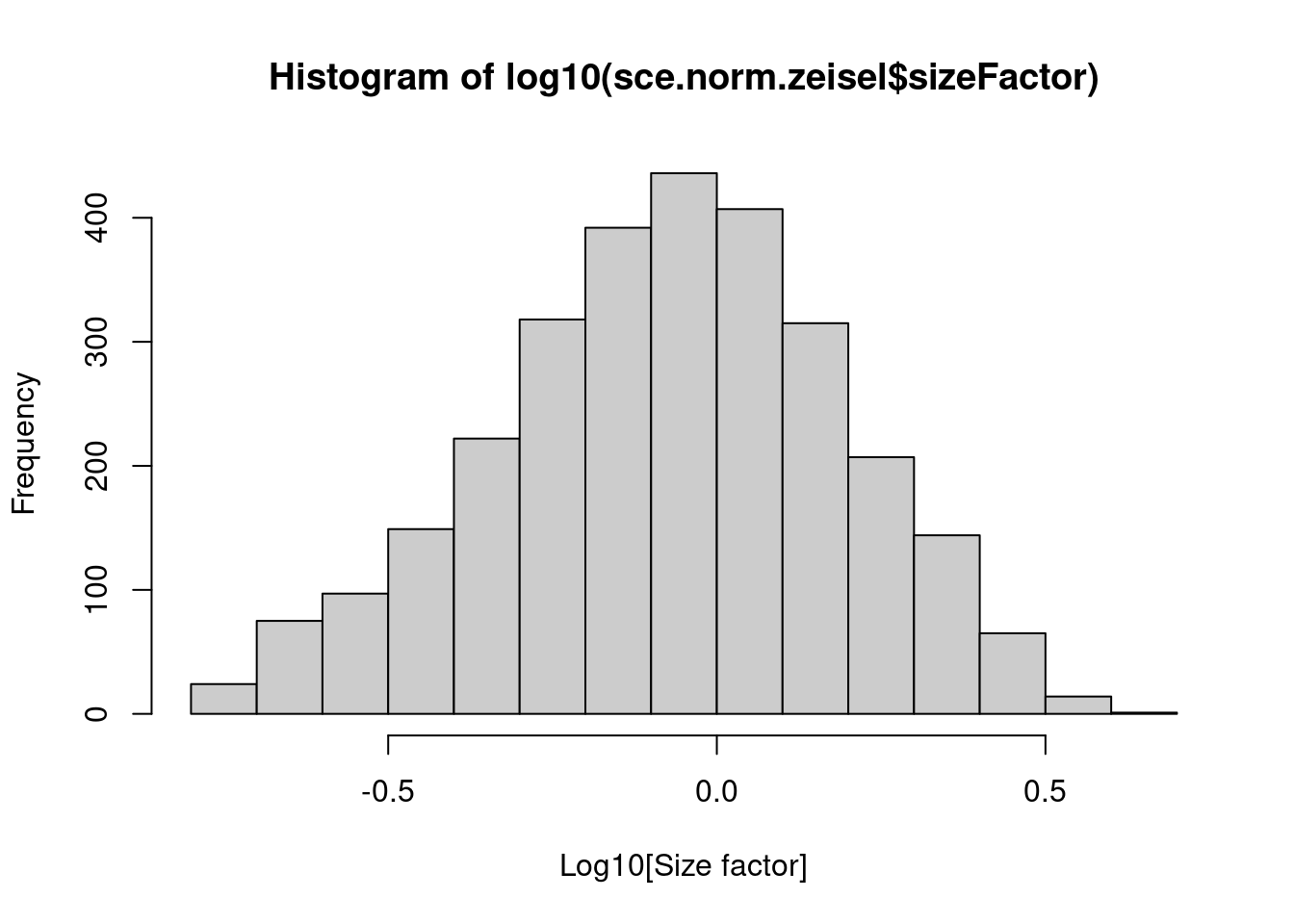
Figure 2.1: Distribution of size factors derived from the library size in the Zeisel brain dataset.
Strictly speaking, the use of library size factors assumes that there is no “imbalance” in the differentially expressed (DE) genes between any pair of cells. That is, any upregulation for a subset of genes is cancelled out by the same magnitude of downregulation in a different subset of genes. This avoids composition biases where upregulation of some genes reduces the sequencing resources available for other genes. If balanced DE is not present, more sophisticated methods for computing size factors may be required (Robinson and Oshlack 2010; Anders and Huber 2010; Lun, Bach, and Marioni 2016). In practice, library size factors perform well for exploratory scRNA-seq data analyses despite their theoretical inaccuracy:
- Gene expression profiles often contain constitutively-expressed genes with large counts, e.g., histones, ribosomal proteins3. These stabilize the library sizes in the presence of imbalanced DE.
- Composition biases do not usually affect the partitioning of cells into clusters (Chapter 6). If the DE was strong enough to introduce a significant composition bias, it is also strong enough to separate the cell subpopulations during clustering.
- Experience from bulk RNA-seq suggests that composition biases are actually quite small, typically introducing a spurious 10-20% difference in expression. This is negligible compared to the order-of-magnitude fold-changes for the marker genes (Chapter 7).
2.3 Normalized expression values
2.3.1 Scaling and log-transforming
The normalizeRnaCounts.se() function uses the size factors to compute normalized expression values from the count matrix.
This is done by dividing all counts for each cell with its corresponding size factor and then applying a log-transformation.
These (log-transformed) normalized expression values will be the basis of our downstream analyses in the following chapters.
logcounts(sce.norm.zeisel)## <20006 x 2866> sparse LogNormalizedMatrix object of type "double":
## 1772071015_C02 1772071017_G12 ... 1772063068_D01 1772066098_A12
## Tspan12 0.0000000 0.0000000 . 0 0
## Tshz1 1.6139535 0.7411389 . 0 0
## Fnbp1l 1.6139535 0.7411389 . 0 0
## Adamts15 0.0000000 0.0000000 . 0 0
## Cldn12 0.7544300 0.7411389 . 0 0
## ... . . . . .
## mt-Co2 5.512629 6.047342 . 7.930569 7.176952
## mt-Co1 5.714860 6.239091 . 8.339569 6.645379
## mt-Rnr2 6.775320 7.780752 . 9.215748 7.486956
## mt-Rnr1 4.478707 5.909090 . 7.274070 5.917989
## mt-Nd4l 3.311873 3.378640 . 5.816615 3.987852The log-transformation is useful as the difference between log-values (i.e., from subtraction) is an estimate of the log-fold change in normalized expression. When comparing expression values, log-fold changes are usually preferable to absolute differences in expression. To illustrate, which one is more interesting - a gene that is expressed at an average count of 50 in cell type \(A\) and 10 in cell type \(B\), or a gene that is expressed at an average count of 1100 in \(A\) and 1000 in \(B\)? Hopefully, we can all agree that the former is more interesting for explaining differences between \(A\) and \(B\). The interpretation of the difference in log-values is important in downstream procedures based on distances between cells, which includes many clustering and dimensionality reduction algorithms. By operating on log-transformed data, we ensure that the distances reflect log-fold changes in expression, e.g., the squared Euclidean distance between two cells is the sum of squared log-fold changes across all genes.
During the log-transformation, normalizeRnaCounts.se() will add a pseudo-count to avoid undefined values at zero counts.
This addition has the side effect of shrinking log-fold changes between cells towards zero for low-abundance genes.
Such shrinkage is desirable as the log-differences are not reliable when the counts are low due to random sampling noise.
So, if we were to use a pseudo-count of 1, the log-fold change between normalized expression values of 1 and 2 would be \(log_2((2 + 1)/(1 + 1)) \approx 0.58\),
while the log-fold change between normalized expression values of 10 and 20 would be \(log_2((20 + 1)/(10 + 1)) \approx 0.93\),
i.e., larger counts will contribute more to the distances between cells.
A pseudo-count of 1 is common for the pragmatic reason that it preserves sparsity, i.e., zeroes in the input remain zeroes after transformation.
However, larger values can also be used for greater shrinkage if low-abundance genes are problematic (Lun 2018).
2.3.2 Why center the size factors?
As previously mentioned, centering ensures that the normalized expression values are on roughly the same scale as the original counts for easier interpretation. For example, Figure 2.2 shows that interneurons have a median Snap25 log-expression from 5 - 6; this roughly translates to an original count of 30 - 60 UMIs in each cell, which gives us some confidence that it is actually expressed. This relationship to the original data would be less obvious if the centering were not performed.
library(scater)
plotExpression(sce.norm.zeisel, x="level1class", features="Snap25", colour="level1class") +
    scale_x_discrete(guide = guide_axis(angle = 45))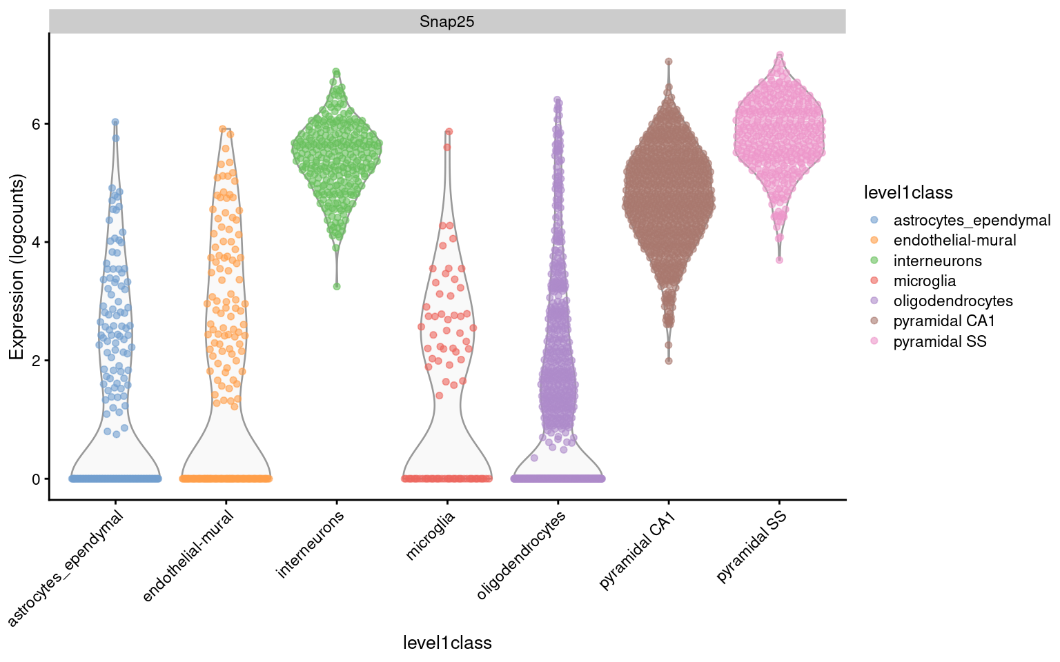
Figure 2.2: Distribution of log-expression values for Snap25 in each cell type of the Zeisel brain dataset.
Centering also ensures that the effect of the pseudo-count decreases with greater sequencing coverage across the dataset. Because we preserve the scale of the input data, the normalized expression values will increase with deeper coverage while the pseudo-count remains the same. This reduces the shrinkage effect and improves the accuracy of the log-fold changes between cells. Which is important, because otherwise, why would we invest in deeper sequencing if our analysis won’t take advantage of it?
For comparison, consider the situation where we applied a constant pseudo-count to some counts-per-million (CPM)-like measure. The accuracy of the subsequent log-fold changes would never improve regardless of how much additional sequencing was performed; scaling to a constant library size of a million means that the pseudo-count will have the same shrinkage effect for all datasets. The same criticism applies to popular metrics like the “counts-per-10K” used in, e.g., seurat. Personally, we rarely use CPM-like measures in scRNA-seq analyses; they are occasionally convenient for rough comparisons between datasets that were processed separately, but in such cases, normalization is the least of our problems (Chapter 8).
2.4 Blocking on experimental batches
Sometimes, our dataset consists of multiple batches of cells that were generated at different sequencing depths. Library size normalization is still applicable but some care is required if the coverage differs dramatically between batches. Specifically, we want to scale down all batches to match the coverage of the lowest-coverage batch. This sacrifices some of the information in high-coverage batches to make them more comparable to the low-coverage batches. By comparison, scaling up the low-coverage batches just amplifies noise as they don’t have the available information to match the high-coverage batches.
Differences in coverage between batches are most obvious when attempting to analyze datasets involving both read and UMI counts5. For two brain datasets generated with different technologies (Zeisel et al. 2015; Tasic et al. 2016), library sizes differ by several orders of magnitude (Figure 2.3). If we scaled up the Zeisel counts by ~100-fold, we would overstate the reliability of low-abundance genes by reducing the pseudo-count shrinkage (Section 2.3.1). This inflates the sampling noise and masks biological signal from higher-abundance genes.
library(scRNAseq)
sce.tasic <- TasicBrainData()
common.brain <- intersect(rownames(sce.zeisel), rownames(sce.tasic))
sce.brain <- combineCols(sce.zeisel[common.brain,], sce.tasic[common.brain,])
sce.brain$study <- rep(c("zeisel", "tasic"), c(ncol(sce.zeisel), ncol(sce.tasic)))

# Batch-specific filters, as discussed in the QC chapter.
# Tasic doesn't have mitochondrial genes so we'll skip that.
library(scrapper)
sce.qc.brain <- quickRnaQc.se(sce.brain, subsets=list(), block=sce.brain$study)
sce.qc.brain <- sce.qc.brain[,sce.qc.brain$keep]

library(scater)
plotColData(sce.qc.brain, x='study', y='sum') + scale_y_log10()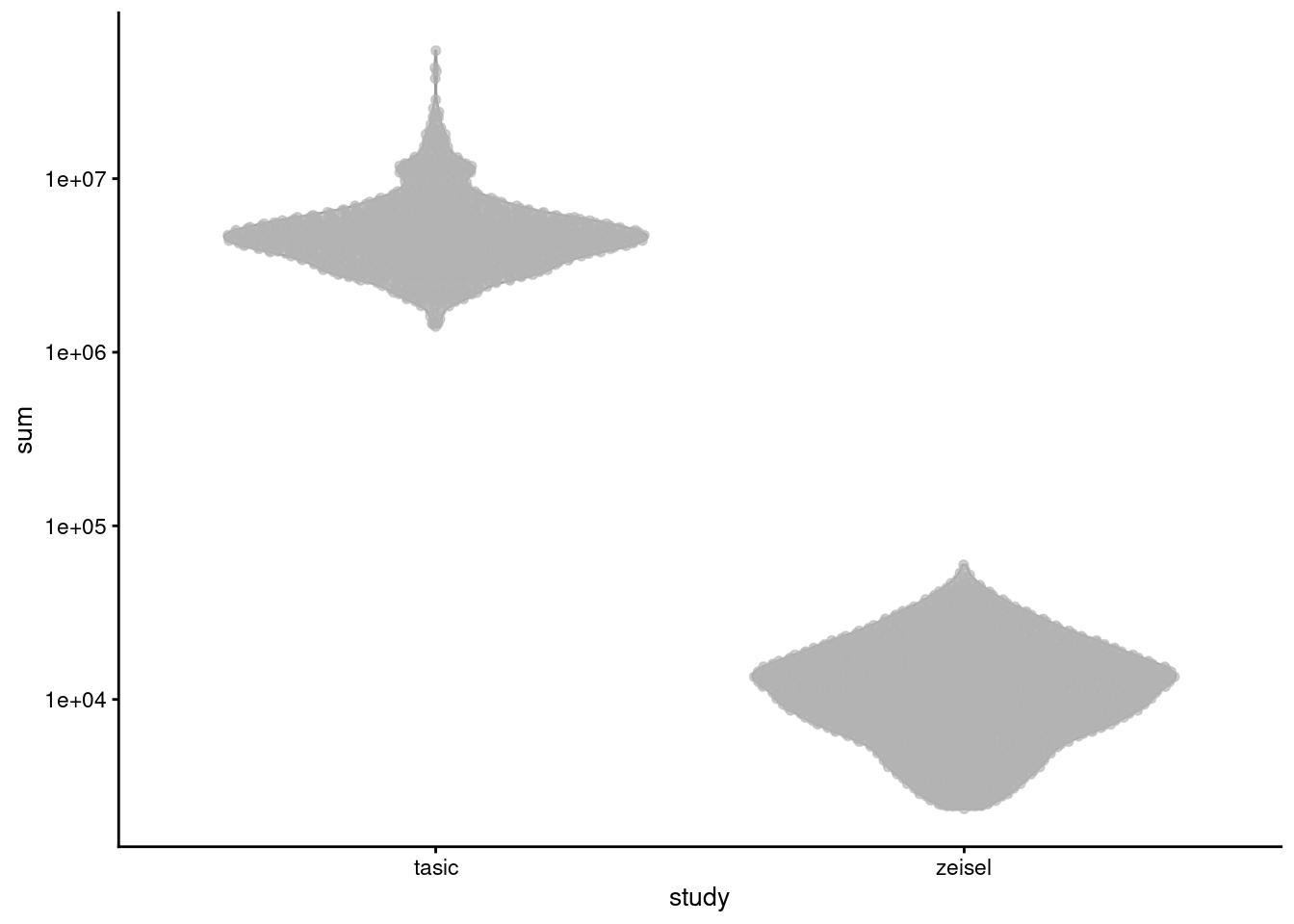
Figure 2.3: Distribution of library sizes for the Tasic and Zeisel brain datasets. Each point represents a cell, separated by the study of origin.
A more conservative approach is to scale down the Tasic counts to match the coverage of the Zeisel data.
We specify the study of origin for each cell in block=, which adjusts the size factors to scale all cells down to the lowest-coverage batch (Figure 2.4).
This avoids amplication of sampling noise at the cost of greater shrinkage when counts are scaled down relative to the pseudo-count (Section 2.3.2).
In effect, we are forcibly reducing the contribution of low-abundance genes in the Tasic data to be consistent with their behavior in the Zeisel data.
Hopefully, there’s still enough signal among the higher-abundance genes to find something interesting in later analysis steps.
sce.norm.brain <- normalizeRnaCounts.se(
    sce.qc.brain,
    size.factors=sce.qc.brain$sum,
    block=sce.qc.brain$study
)

plotColData(sce.norm.brain, x='study', y='sizeFactor') +
    geom_hline(yintercept=1, linetype="dashed", color="red") +
    scale_y_log10()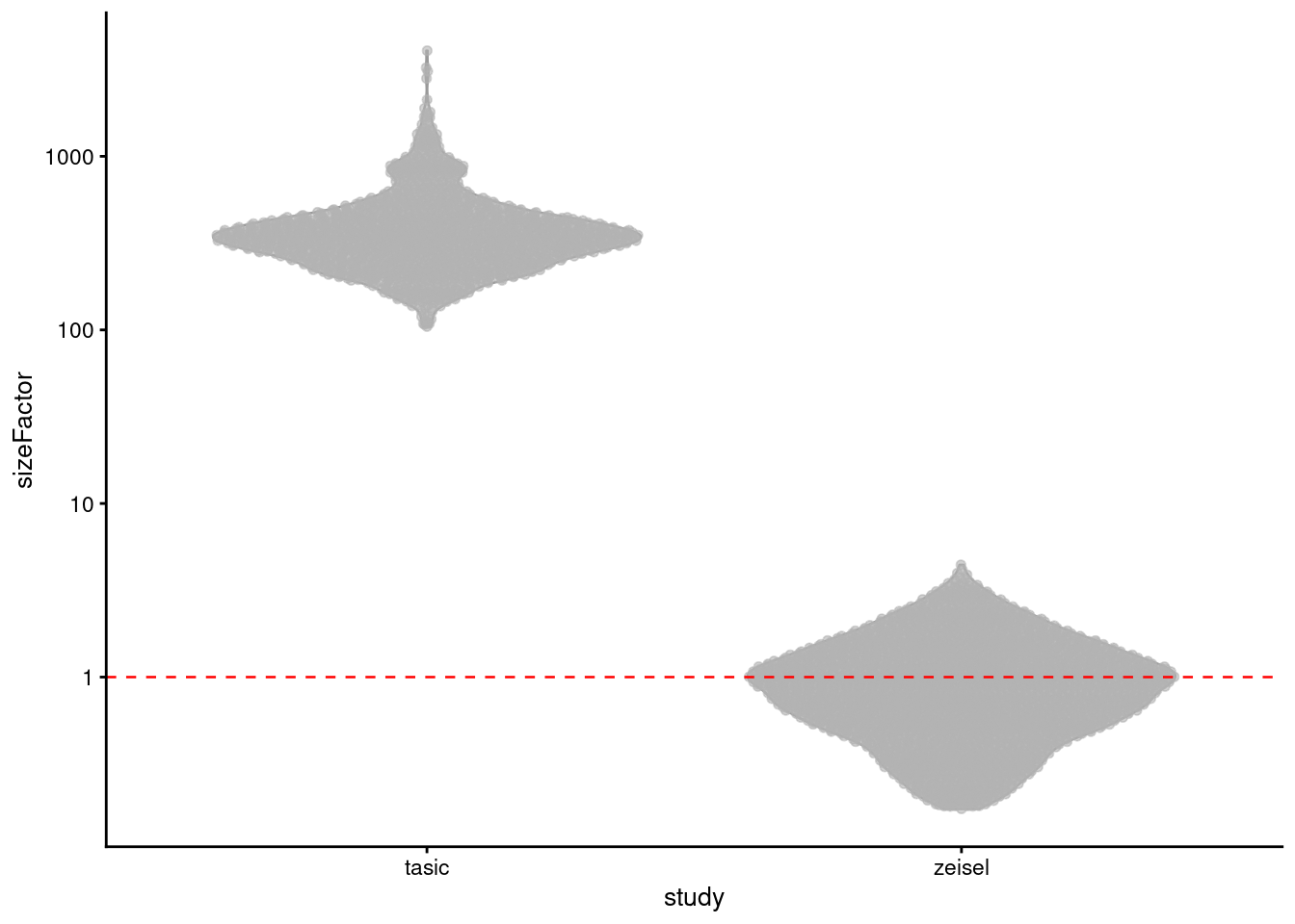
Figure 2.4: Distribution of block-centered size factors for the Tasic and Zeisel brain datasets. Each point represents a cell, separated by the study of origin.
Note that our batch-aware normalization is not the same as batch correction.
The former will only remove scaling biases between cells whereas the latter considers more potential axes of uninteresting variation between batches.
For example, differences in processing of one batch may result in more or less activity in certain pathways that cannot be removed with per-cell scaling factors.
Normalization with block= is still helpful as it eliminates one of the differences between batches,
but it usually needs to be followed by more sophisticated methods (Chapter 8) to avoid batch effects in later analysis steps.
2.5 Normalization by spike-ins
Occasionally, we might come across an scRNA-seq dataset with spike-in counts, which gives us the opportunity to perform spike-in normalization (A. T. L. Lun et al. 2017)6. This assumes that (i) the same amount of spike-in RNA was added to each cell and (ii) the spike-in transcripts respond to experimental biases in the same relative manner as endogenous genes. Thus, any systematic difference in the coverage of the spike-in transcripts can attributed to cell-specific biases, e.g., in capture efficiency or sequencing depth. To remove these biases, we equalize spike-in coverage across cells by scaling with “spike-in size factors”.
Let’s demonstrate on a scRNA-seq dataset of T cells after stimulation with T cell receptor ligands of varying affinity (Richard et al. 2018).
Specifically, we compute the total count across all spike-in transcripts in each cell and center them to a mean of 1 across all cells (see Section 2.3.2).
These size factors can then be plugged into normalizeRnaCounts.se() to obtain normalized expression values for endogenous genes.
library(scRNAseq)
sce.richard <- RichardTCellData()

# For brevity, we'll just re-use the authors' QC calls.
sce.qc.richard <- sce.richard[,sce.richard$`single cell quality`=="OK"]
sce.qc.richard
## class: SingleCellExperiment
## dim: 46603 528
## metadata(0):
## assays(1): counts
## rownames(46603): ENSMUSG00000102693 ENSMUSG00000064842 ...
## ENSMUSG00000096730 ENSMUSG00000095742
## rowData names(0):
## colnames(528): SLX-12611.N701_S502. SLX-12611.N702_S502. ...
## SLX-12612.i712_i522. SLX-12612.i714_i522.
## colData names(13): age individual ... stimulus time
## reducedDimNames(0):
## mainExpName: endogenous
## altExpNames(1): ERCC# Pulling the spike-in counts out of the alternative experiment.
sce.ercc.richard <- altExp(sce.qc.richard, "ERCC")
sce.ercc.richard## class: SingleCellExperiment
## dim: 92 528
## metadata(0):
## assays(1): counts
## rownames(92): ERCC-00002 ERCC-00003 ... ERCC-00170 ERCC-00171
## rowData names(3): subgroup concentration molecules
## colnames(528): SLX-12611.N701_S502. SLX-12611.N702_S502. ...
## SLX-12612.i712_i522. SLX-12612.i714_i522.
## colData names(0):
## reducedDimNames(0):
## mainExpName: NULL
## altExpNames(0):library(scrapper)
ercc.sums.richard <- colSums(counts(sce.ercc.richard))
spike.factor.richard <- centerSizeFactors(ercc.sums.richard)
summary(spike.factor.richard)## Min. 1st Qu. Median Mean 3rd Qu. Max.
## 0.1247 0.4282 0.6274 1.0000 1.0699 23.3161hist(log10(spike.factor.richard), xlab="Log10[Size factor]", col='grey80')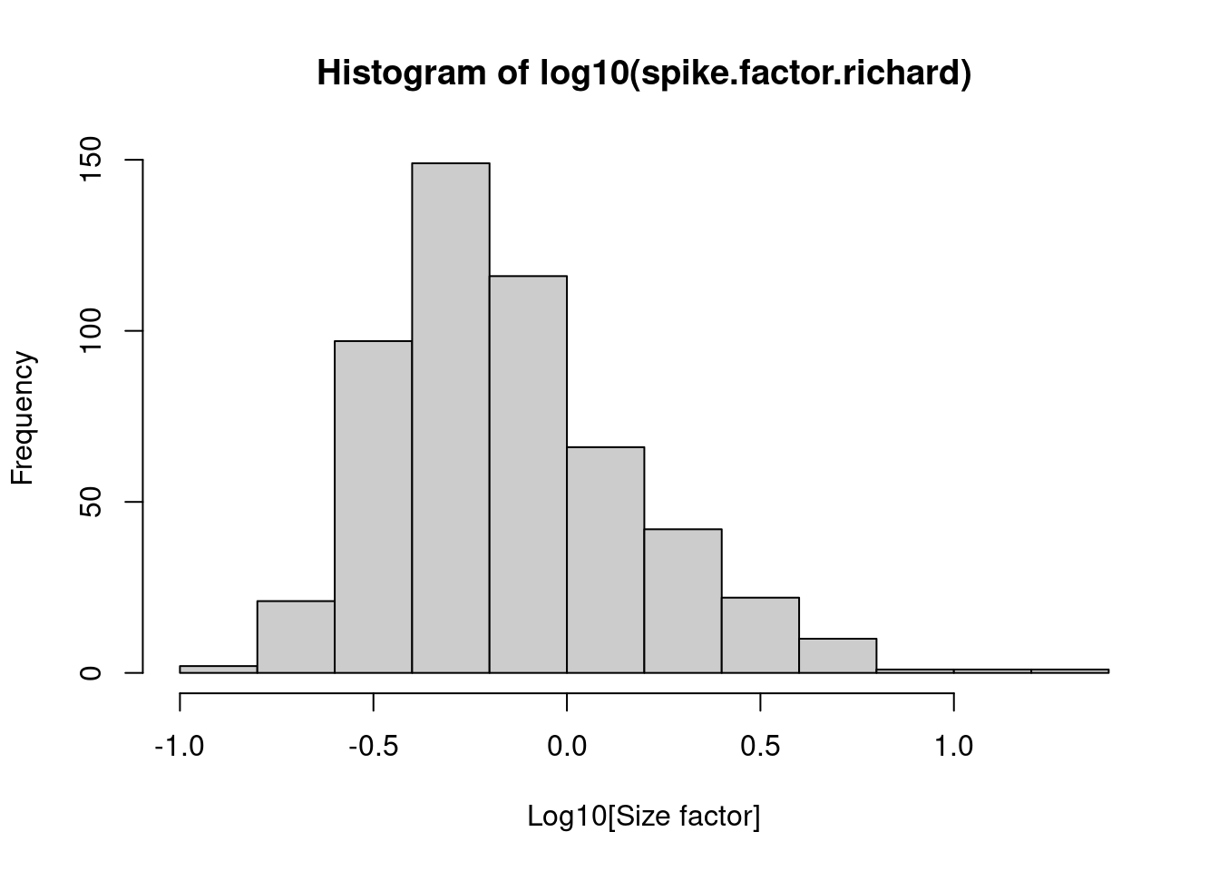
Figure 2.5: Distribution of size factors derived from the library size in the Richard T cell dataset.
Practically, spike-in normalization should be used if differences in the total RNA content between cells are of interest and must be preserved in downstream analyses. For a given cell, an increase in its overall amount of endogenous RNA will not increase its spike-in size factor. This ensures that the effects of total RNA content on expression across the population will not be removed upon scaling. By comparison, library size normalization will consider any change in total RNA content as part of the bias and remove it.
The differences between these two normalization strategies in illustrated in Figure 2.6. The spike-in size factors and deconvolution size factors are positively correlated within each treatment condition, indicating that they are capturing similar technical biases in sequencing depth and capture efficiency. However, increasing stimulation of the T cell receptor (in terms of increasing affinity or time) results in a decrease in the spike-in factors relative to the library size factors. This is consistent with an increase in total RNA content during stimulation, which increases the coverage of endogenous genes at the expense of the spike-in transcripts.
rna.sums.richard <- colSums(counts(sce.qc.richard))
lib.factor.richard <- centerSizeFactors(rna.sums.richard)
to.plot <- data.frame(
    LibFactor=lib.factor.richard,
    SpikeFactor=spike.factor.richard,
    Stimulus=sce.qc.richard$stimulus,
    Time=sce.qc.richard$time
)

library(ggplot2)
ggplot(to.plot, aes(x=LibFactor, y=SpikeFactor, color=Time)) +
    geom_point() +
    facet_wrap(~Stimulus) +
    scale_x_log10() +
    scale_y_log10() +
    geom_abline(intercept=0, slope=1, color="red")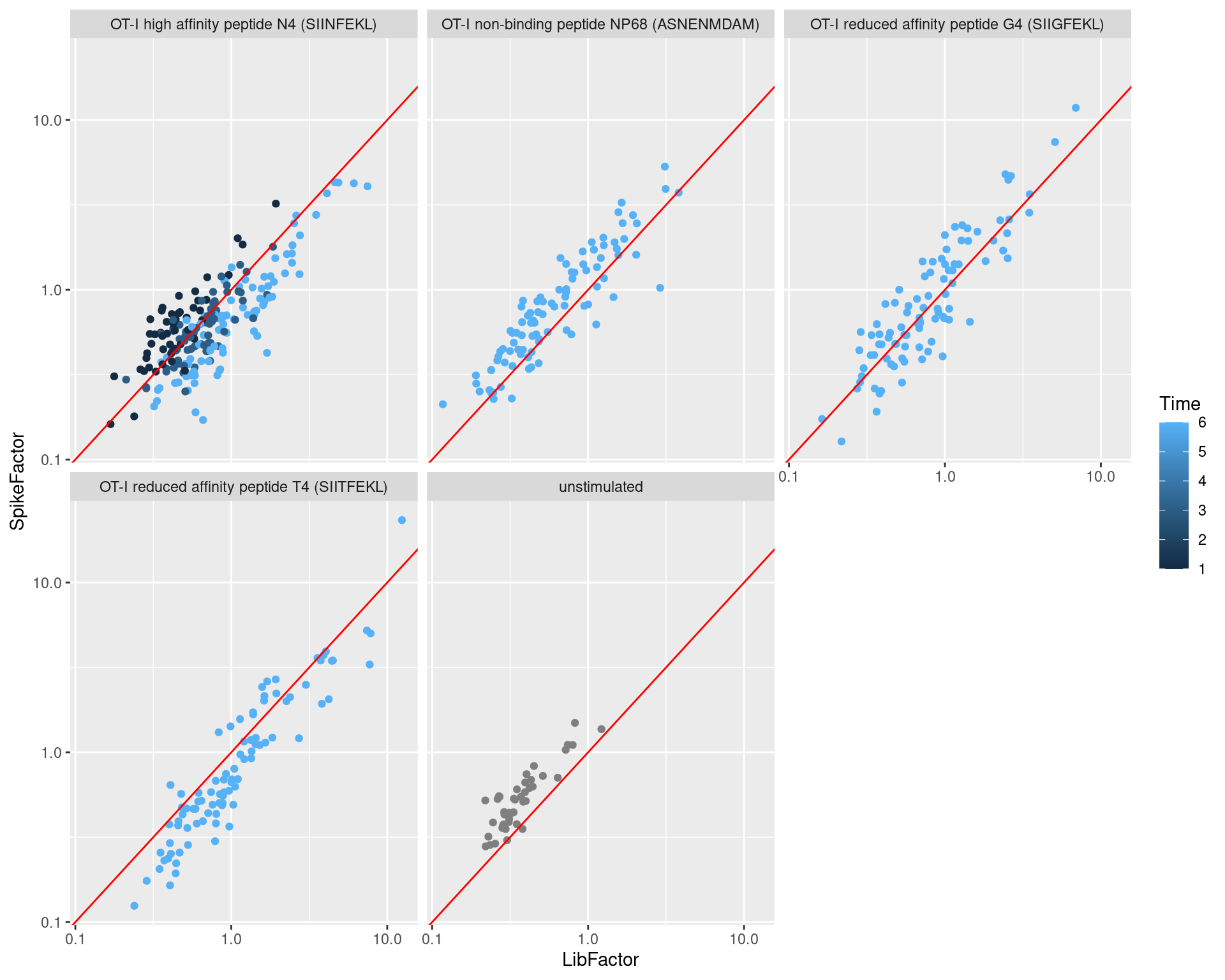
Figure 2.6: Size factors from spike-in normalization, plotted against the library size factors for all cells in the T cell dataset. Each plot represents a different ligand treatment and each point is a cell coloured according by time from stimulation.
These differences have real consequences for downstream interpretation. If the spike-in size factors were applied to the counts, the expression values in unstimulated cells would be scaled up while expression in stimulated cells would be scaled down. However, the opposite would occur if the deconvolution size factors were used. This can manifest as shifts in the magnitude and direction of DE between conditions when we switch between normalization strategies, as shown below for our most beloved gene Malat1 (Figure 2.7).
# Setting center=FALSE because we already centered the size factors.
sce.lib.richard <- normalizeRnaCounts.se(sce.qc.richard, size.factors=lib.factor.richard, center=FALSE)
sce.spike.richard <- normalizeRnaCounts.se(sce.qc.richard, size.factors=spike.factor.richard, center=FALSE)

library(scater)
gridExtra::grid.arrange(
    plotExpression(sce.lib.richard, x="stimulus", colour_by="time", features="ENSMUSG00000092341") +
        scale_x_discrete(guide = guide_axis(angle = 70)) +
        ggtitle("After library size normalization"),
    plotExpression(sce.spike.richard, x="stimulus", colour_by="time", features="ENSMUSG00000092341") +
        scale_x_discrete(guide = guide_axis(angle = 70)) +
        ggtitle("After spike-in normalization"),
    ncol=2
)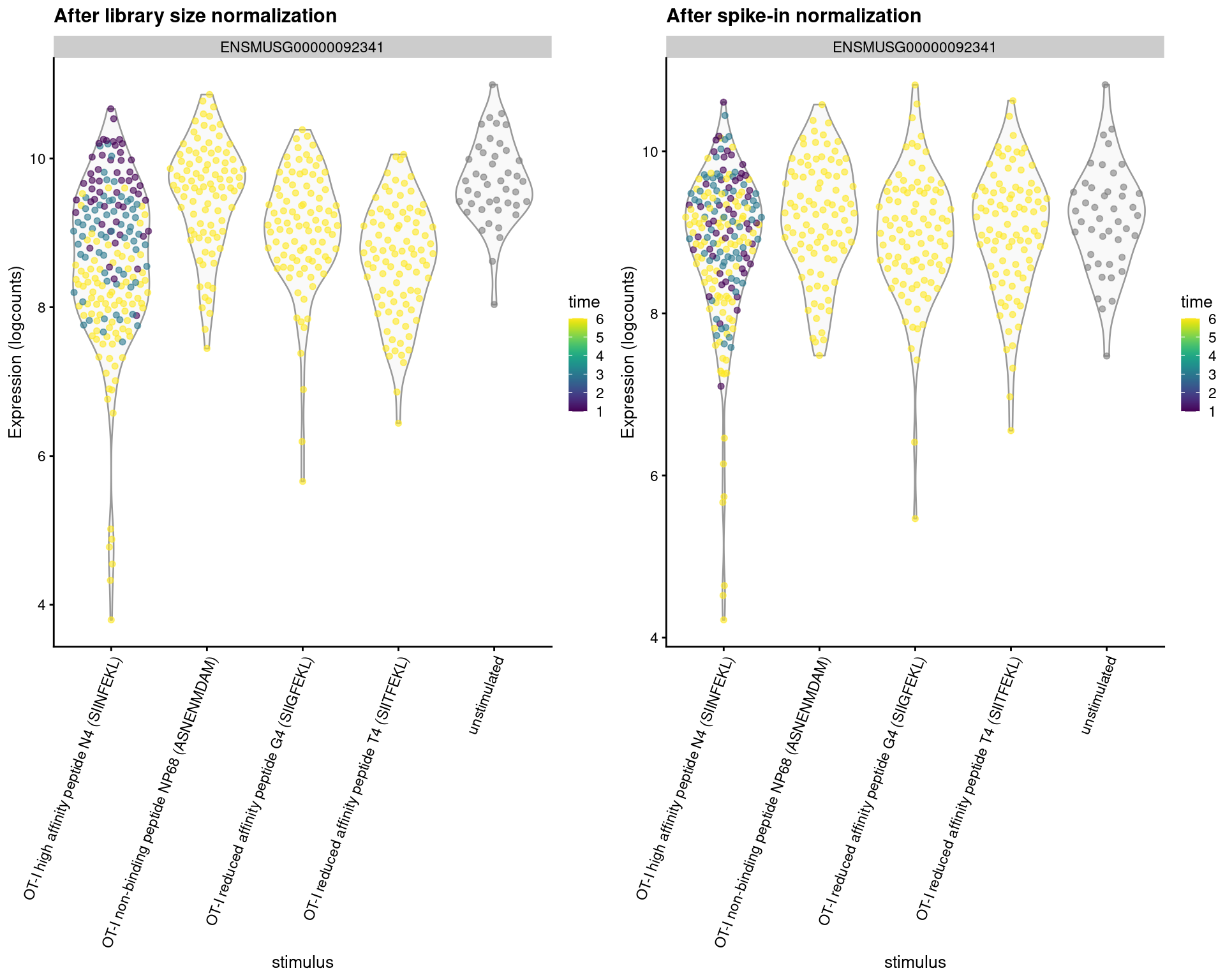
Figure 2.7: Distribution of log-normalized expression values for Malat1 after normalization with the deconvolution size factors (left) or spike-in size factors (right). Cells are stratified by the ligand affinity and colored by the time after stimulation.
Whether or not total RNA content is relevant – and thus, the choice of normalization strategy – depends on the biological hypothesis. In most cases, changes in total RNA content are not interesting and can be normalized out with the library size factors. However, this may not always be appropriate if differences in total RNA are associated with a biological process of interest, e.g., cell cycle activity or T cell activation. Spike-in normalization will preserve these differences such that any changes in expression between biological groups have the correct sign.
Session information
sessionInfo()## R Under development (unstable) (2025-12-24 r89227)
## Platform: x86_64-pc-linux-gnu
## Running under: Ubuntu 22.04.5 LTS
##
## Matrix products: default
## BLAS: /home/luna/Software/R/trunk/lib/libRblas.so
## LAPACK: /home/luna/Software/R/trunk/lib/libRlapack.so; LAPACK version 3.12.1
##
## locale:
## [1] LC_CTYPE=en_US.UTF-8 LC_NUMERIC=C
## [3] LC_TIME=en_US.UTF-8 LC_COLLATE=en_US.UTF-8
## [5] LC_MONETARY=en_US.UTF-8 LC_MESSAGES=en_US.UTF-8
## [7] LC_PAPER=en_US.UTF-8 LC_NAME=C
## [9] LC_ADDRESS=C LC_TELEPHONE=C
## [11] LC_MEASUREMENT=en_US.UTF-8 LC_IDENTIFICATION=C
##
## time zone: Australia/Sydney
## tzcode source: system (glibc)
##
## attached base packages:
## [1] stats4 stats graphics grDevices utils datasets methods
## [8] base
##
## other attached packages:
## [1] ensembldb_2.35.0 AnnotationFilter_1.35.0
## [3] GenomicFeatures_1.63.1 AnnotationDbi_1.73.0
## [5] scater_1.39.1 ggplot2_4.0.1
## [7] scuttle_1.21.0 scrapper_1.5.10
## [9] scRNAseq_2.25.0 SingleCellExperiment_1.33.0
## [11] SummarizedExperiment_1.41.0 Biobase_2.71.0
## [13] GenomicRanges_1.63.1 Seqinfo_1.1.0
## [15] IRanges_2.45.0 S4Vectors_0.49.0
## [17] BiocGenerics_0.57.0 generics_0.1.4
## [19] MatrixGenerics_1.23.0 matrixStats_1.5.0
## [21] BiocStyle_2.39.0
##
## loaded via a namespace (and not attached):
## [1] RColorBrewer_1.1-3 jsonlite_2.0.0 magrittr_2.0.4
## [4] ggbeeswarm_0.7.3 gypsum_1.7.0 farver_2.1.2
## [7] rmarkdown_2.30 BiocIO_1.21.0 vctrs_0.6.5
## [10] memoise_2.0.1 Rsamtools_2.27.0 RCurl_1.98-1.17
## [13] htmltools_0.5.9 S4Arrays_1.11.1 AnnotationHub_4.1.0
## [16] curl_7.0.0 BiocNeighbors_2.5.0 Rhdf5lib_1.33.0
## [19] SparseArray_1.11.10 rhdf5_2.55.12 sass_0.4.10
## [22] alabaster.base_1.11.1 bslib_0.9.0 alabaster.sce_1.11.0
## [25] httr2_1.2.2 cachem_1.1.0 GenomicAlignments_1.47.0
## [28] lifecycle_1.0.5 pkgconfig_2.0.3 rsvd_1.0.5
## [31] Matrix_1.7-4 R6_2.6.1 fastmap_1.2.0
## [34] digest_0.6.39 irlba_2.3.5.1 ExperimentHub_3.1.0
## [37] RSQLite_2.4.5 beachmat_2.27.1 labeling_0.4.3
## [40] filelock_1.0.3 httr_1.4.7 abind_1.4-8
## [43] compiler_4.6.0 bit64_4.6.0-1 withr_3.0.2
## [46] S7_0.2.1 BiocParallel_1.45.0 viridis_0.6.5
## [49] DBI_1.2.3 HDF5Array_1.39.0 alabaster.ranges_1.11.0
## [52] alabaster.schemas_1.11.0 rappdirs_0.3.3 DelayedArray_0.37.0
## [55] rjson_0.2.23 tools_4.6.0 vipor_0.4.7
## [58] otel_0.2.0 beeswarm_0.4.0 glue_1.8.0
## [61] h5mread_1.3.1 restfulr_0.0.16 rhdf5filters_1.23.3
## [64] grid_4.6.0 gtable_0.3.6 BiocSingular_1.27.1
## [67] ScaledMatrix_1.19.0 XVector_0.51.0 ggrepel_0.9.6
## [70] BiocVersion_3.23.1 pillar_1.11.1 dplyr_1.1.4
## [73] BiocFileCache_3.1.0 lattice_0.22-7 rtracklayer_1.71.3
## [76] bit_4.6.0 tidyselect_1.2.1 Biostrings_2.79.4
## [79] knitr_1.51 gridExtra_2.3 bookdown_0.46
## [82] ProtGenerics_1.43.0 xfun_0.55 UCSC.utils_1.7.1
## [85] lazyeval_0.2.2 yaml_2.3.12 evaluate_1.0.5
## [88] codetools_0.2-20 cigarillo_1.1.0 tibble_3.3.0
## [91] alabaster.matrix_1.11.0 BiocManager_1.30.27 cli_3.6.5
## [94] jquerylib_0.1.4 dichromat_2.0-0.1 Rcpp_1.1.1
## [97] GenomeInfoDb_1.47.2 dbplyr_2.5.1 png_0.1-8
## [100] XML_3.99-0.20 parallel_4.6.0 blob_1.2.4
## [103] bitops_1.0-9 viridisLite_0.4.2 alabaster.se_1.11.0
## [106] scales_1.4.0 purrr_1.2.1 crayon_1.5.3
## [109] rlang_1.1.7 cowplot_1.2.0 KEGGREST_1.51.1References
Anders, S., and W. Huber. 2010. “Differential expression analysis for sequence count data.” Genome Biol. 11 (10): R106.
Lun, A. 2018. “Overcoming Systematic Errors Caused by Log-Transformation of Normalized Single-Cell Rna Sequencing Data.” bioRxiv.
Lun, A. T., K. Bach, and J. C. Marioni. 2016. “Pooling across cells to normalize single-cell RNA sequencing data with many zero counts.” Genome Biol. 17 (April): 75.
Lun, A. T. L., F. J. Calero-Nieto, L. Haim-Vilmovsky, B. Gottgens, and J. C. Marioni. 2017. “Assessing the reliability of spike-in normalization for analyses of single-cell RNA sequencing data.” Genome Res. 27 (11): 1795–1806.
Marioni, J. C., C. E. Mason, S. M. Mane, M. Stephens, and Y. Gilad. 2008. “RNA-seq: an assessment of technical reproducibility and comparison with gene expression arrays.” Genome Res. 18 (9): 1509–17.
Richard, A. C., A. T. L. Lun, W. W. Y. Lau, B. Gottgens, J. C. Marioni, and G. M. Griffiths. 2018. “T cell cytolytic capacity is independent of initial stimulation strength.” Nat. Immunol. 19 (8): 849–58.
Robinson, M. D., and A. Oshlack. 2010. “A scaling normalization method for differential expression analysis of RNA-seq data.” Genome Biol. 11 (3): R25.
Stegle, O., S. A. Teichmann, and J. C. Marioni. 2015. “Computational and analytical challenges in single-cell transcriptomics.” Nat. Rev. Genet. 16 (3): 133–45.
Tasic, B., V. Menon, T. N. Nguyen, T. K. Kim, T. Jarsky, Z. Yao, B. Levi, et al. 2016. “Adult mouse cortical cell taxonomy revealed by single cell transcriptomics.” Nat. Neurosci. 19 (2): 335–46.
Zeisel, A., A. B. Munoz-Manchado, S. Codeluppi, P. Lonnerberg, G. La Manno, A. Jureus, S. Marques, et al. 2015. “Brain structure. Cell types in the mouse cortex and hippocampus revealed by single-cell RNA-seq.” Science 347 (6226): 1138–42.
2.3.3 Comments on other transformations
We might see a variety of other transformations in the wild:
DESeq2::vst()or sctransform, which aim to remove the mean-variance dependency in (sc)RNA-seq count data. This ensures that genes of varying abundance contribute equally to downstream analyses. However, stabilization is challenging in heterogeneous datasets where biological variation interferes with the distributional assumptions of these methods.In practice, the log-transformation is a good default choice due to its simplicity and interpretability, and is what we will be using for all downstream analyses.