Chapter 9 Protein multiomics
9.1 Motivation
Cellular indexing of transcriptomes and epitopes by sequencing (CITE-seq) simultaneously quantifies gene expression and surface protein abundance in each cell (Stoeckius et al. 2017). First, we create antibodies against the proteins of interest and conjugate them to synthetic RNA tags, i.e., antibody-derived tags (ADTs)35. Cells are labelled with these antibodies and processed with single-cell technologies like 10X Genomics. For each cell, both ADTs and endogenous transcripts are reverse-transcribed into cDNA and sequenced. This yields a set of counts for the ADTs, to quantify the abundance of each selected protein; and another set of counts for the genes, as in scRNA-seq. We can then examine aspects of the proteome (e.g., post-translational modifications) and other cellular features that would normally be overlooked in transcriptomic studies.
To analyze CITE-seq data, we split the dataset into the RNA and ADT counts and apply usual steps (quality control, normalization, etc.) to each modality. For the RNA modality, we can re-use the same functions from the previous chapters as if the data were generated from an scRNA-seq experiment. For ADTs, some tweaks are necessary to account for unique aspects of the ADT counts - specifically, fewer features are available as the proteins of interest were chosen by the reseacher, and the coverage of each ADT is much deeper as the sequencing resources are concentrated into a smaller number of features. Once modality-specific processing is complete, we combine the ADT and RNA data so that information in both modalities are used in downstream steps like clustering.
9.2 Quality control
As in the RNA-based analysis, we want to remove cells in which ADTs were not efficiently captured or sequenced. This involves similar QC metrics to those described in Chapter 1, specifically:
- The number of ADTs detected (i.e., with non-zero counts) in each cell. We expect non-zero counts for most ADTs in each cell, even if the corresponding protein target is not present on the cell surface. This is due to deeper sequencing coverage that detects up free-floating antibodies in the ambient solution or antibodies that are non-specifically bound to the cell membrance. An unusually low number of detected features is indicative of a failure in library preparation or sequencing.
- The sum of counts for isotype control (IgG) antibodies. IgG controls lack a specific target in the cell but otherwise have similar properties to the primary antibodies against the proteins of interest. The coverage of these control ADTs serves as a measure of non-specific binding in each cell. A large sum for the controls is indicative of a problem with specificity, possibly even the formation of undesirable protein aggregates.
We demonstrate using a PBMC dataset from 10X Genomics (Zheng et al. 2017) that contains quantified abundances for a number of interesting surface proteins.
library(DropletTestFiles)
path.pbmc <- getTestFile("tenx-3.0.0-pbmc_10k_protein_v3/1.0.0/filtered.tar.gz")
dir.pbmc <- tempfile()
untar(path.pbmc, exdir=dir.pbmc)

# Loading it in as a SingleCellExperiment object.
library(DropletUtils)
sce.pbmc <- read10xCounts(file.path(dir.pbmc, "filtered_feature_bc_matrix"))

# Splitting off the ADTs into an alternative experiment for separate
# processing, otherwise they'd be treated as genes.
sce.pbmc <- splitAltExps(sce.pbmc, rowData(sce.pbmc)$Type)
sce.pbmc
## class: SingleCellExperiment
## dim: 33538 7865
## metadata(1): Samples
## assays(1): counts
## rownames(33538): ENSG00000243485 ENSG00000237613 ... ENSG00000277475
## ENSG00000268674
## rowData names(3): ID Symbol Type
## colnames: NULL
## colData names(2): Sample Barcode
## reducedDimNames(0):
## mainExpName: Gene Expression
## altExpNames(1): Antibody Capture# Here, the "main" experiment contains the RNA data, while the alternative
# experiment contains the antibody data.
mainExpName(sce.pbmc)## [1] "Gene Expression"sce.adt.pbmc <- altExp(sce.pbmc, "Antibody Capture")
sce.adt.pbmc## class: SingleCellExperiment
## dim: 17 7865
## metadata(1): Samples
## assays(1): counts
## rownames(17): CD3 CD4 ... IgG1 IgG2b
## rowData names(3): ID Symbol Type
## colnames: NULL
## colData names(0):
## reducedDimNames(0):
## mainExpName: NULL
## altExpNames(0):# Taking a sneak peak at the ADT counts.
counts(sce.adt.pbmc)[,1:10]## 17 x 10 sparse Matrix of class "dgCMatrix"
##
## CD3 18 30 18 18 5 21 34 48 4522 2910
## CD4 138 119 207 11 14 1014 324 1127 3479 2900
## CD8a 13 19 10 17 14 29 27 43 38 28
## CD14 491 472 1289 20 19 2428 1958 2189 55 41
## CD15 61 102 128 124 156 204 607 128 111 130
## CD16 17 155 72 1227 1873 148 676 75 44 37
## CD56 17 248 26 491 458 29 29 29 30 15
## CD19 3 3 8 5 4 7 15 4 6 6
## CD25 9 5 15 15 16 52 85 17 13 18
## CD45RA 110 125 5268 4743 4108 227 175 523 4044 1081
## CD45RO 74 156 28 28 21 492 517 316 26 43
## PD-1 9 9 20 25 28 16 26 16 28 16
## TIGIT 4 9 11 59 76 11 12 12 9 8
## CD127 7 8 12 16 17 15 11 10 231 179
## IgG2a 5 4 12 12 7 9 6 3 19 14
## IgG1 2 8 19 16 14 10 12 7 16 10
## IgG2b 3 3 6 4 9 8 50 2 8 2We compute each of the QC metrics described above from the ADT count matrix. We also compute the sum of counts across all ADTs for each cell, but this is strictly for informational purposes only as it is not an effective QC metric. Specifically, the presence of a targeted protein can lead to a several-fold increase in the total ADT count, given the binary nature of most surface markers. Removing cells with low total ADT counts could inadvertently eliminate cell types that do not express many - or indeed, any - of the selected protein targets. Similarly, we prefer to use the sum of IgG counts instead of the proportion as the latter relies on the total count and is more affected by the biology. For example, a cell that does not express any of the targets would have a lower total and thus a higher IgG proportion, making it unfairly susceptible to removal.
library(scrapper)
is.igg.pbmc <- grep("^IgG", rownames(sce.adt.pbmc))
sce.qc.adt.pbmc <- quickAdtQc.se(sce.adt.pbmc, subsets=list(IgG=is.igg.pbmc))
summary(sce.qc.adt.pbmc$sum)
## Min. 1st Qu. Median Mean 3rd Qu. Max.
## 0 3332 5816 6509 8166 147076summary(sce.qc.adt.pbmc$detected)## Min. 1st Qu. Median Mean 3rd Qu. Max.
## 0.00 17.00 17.00 16.94 17.00 17.00summary(sce.qc.adt.pbmc$subset.sum.IgG)## Min. 1st Qu. Median Mean 3rd Qu. Max.
## 0.00 18.00 23.00 27.41 30.00 2113.00The quickAdtQc.se() function computes thresholds using the outlier-based strategy described in Section 1.3.1 (Figure 9.1).
We use a log-transformation for the number of detected features and the IgG sum to avoid negative thresholds and improve normality.
We also perform a minor adjustment to relax the threshold for the number of detected ADTs if the MAD is zero.
qc.thresh.adt.pbmc <- metadata(sce.qc.adt.pbmc)$qc$thresholds
qc.thresh.adt.pbmc
## $detected
## [1] 15.3
##
## $subset.sum
## IgG
## 74.98505library(scater)
gridExtra::grid.arrange(
plotColData(sce.qc.adt.pbmc, y="detected") +
geom_hline(yintercept=qc.thresh.adt.pbmc$detected, linetype="dashed", color="red") +
ggtitle("Detected features"),
plotColData(sce.qc.adt.pbmc, y="subset.sum.IgG") +
geom_hline(yintercept=qc.thresh.adt.pbmc$subset.sum["IgG"], linetype="dashed", color="red") +
scale_y_log10() +
ggtitle("IgG sum"),
ncol=2
)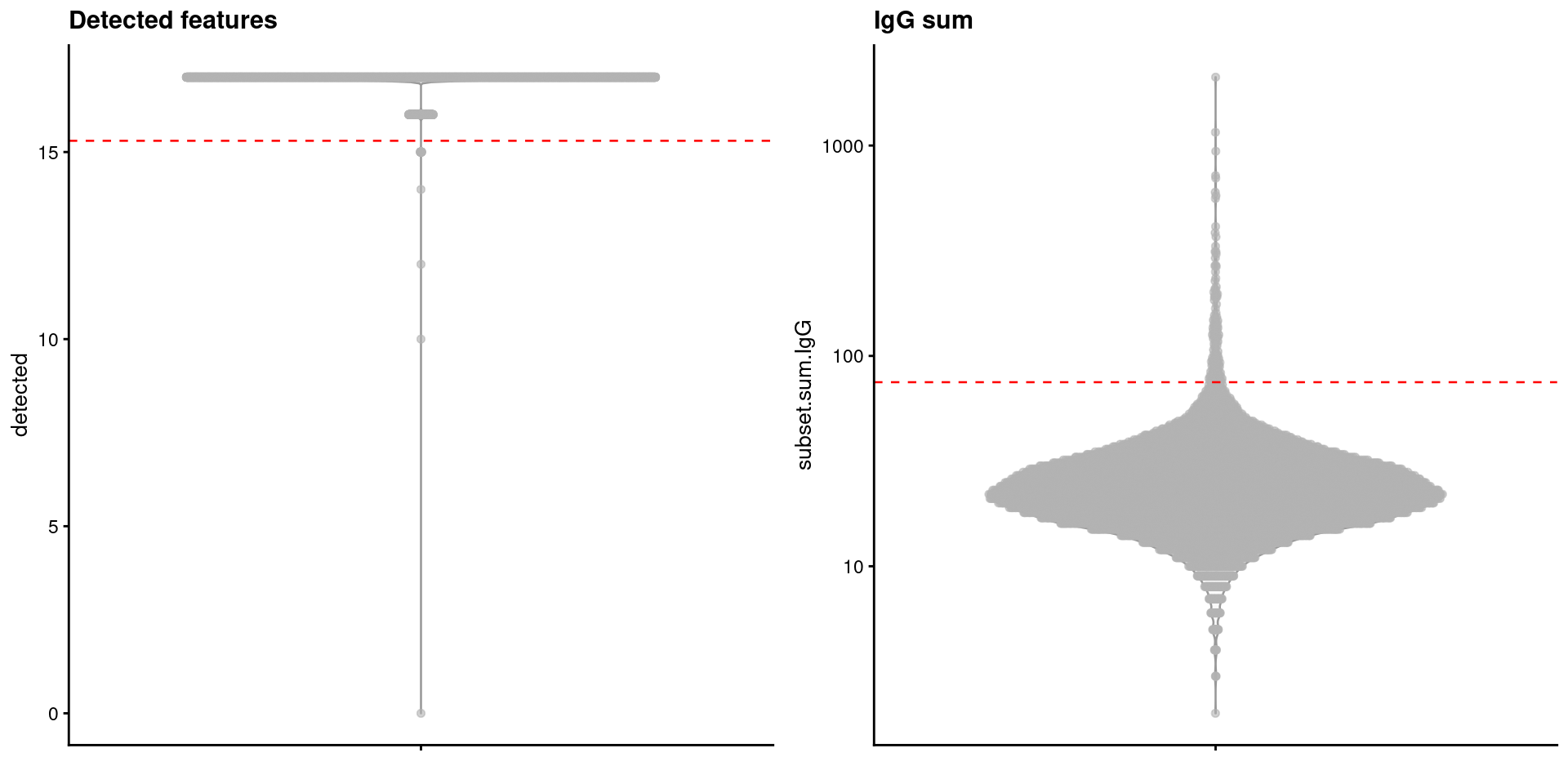
Figure 9.1: Distribution of ADT-based QC metrics in the PBMC dataset. Each point represents a cell, while dashed lines represent thresholds for each metric.
We then apply these thresholds to our metrics to identify high-quality cells. If we wanted to use custom thresholds, we could modify our thresholds in the same manner as described in Section 1.3.2. Similarly, if our dataset contained multiple experimental batches, we could use the same blocking approach as described in Section 1.5.
summary(sce.qc.adt.pbmc$keep)## Mode FALSE TRUE
## logical 158 7707If we were only interested in the ADT data, we could subset our SingleCellExperiment with qc.keep.adt.pbmc and proceed to the next step.
However, the entire purpose of CITE-seq is to examine both protein abundance and gene expression for the same cell.
Thus, we need to apply quality control to the RNA counts as described in Chapter 1.
We only keep cells that are considered to be of high quality in both of the ADT and RNA modalities.
is.mito.pbmc <- grep("^MT-", rowData(sce.pbmc)$Symbol)
sce.qc.pbmc <- quickRnaQc.se(sce.pbmc, subsets=list(MT=is.mito.pbmc))

# Seeing how many cells pass both, one or neither QC filters.
table(RNA=sce.qc.pbmc$keep, ADT=sce.qc.adt.pbmc$keep)
## ADT
## RNA FALSE TRUE
## FALSE 41 296
## TRUE 117 7411# Only keeping cells that pass both filters.
qc.keep.combined.pbmc <- sce.qc.pbmc$keep & sce.qc.adt.pbmc$keep
sce.qc.pbmc <- sce.qc.pbmc[,qc.keep.combined.pbmc]
sce.qc.adt.pbmc <- sce.qc.adt.pbmc[,qc.keep.combined.pbmc]
ncol(sce.qc.pbmc)## [1] 74119.3 Normalization
As with RNA, we performing scaling normalization to remove cell-specific biases due to differences in library preparation and sequencing efficiency (Chapter 2). Unfortunately, we can’t just take the size factors for the RNA counts and re-use them for the ADTs. The two modalities will be subject to different biases due to differences in biophysical properties between endogenous transcripts and ADTs, e.g., length, sequence composition. Some aspects of the library preparation and sequencing are also unique to each modality, providing more opportunities for differences in the biases. So, instead, we need to compute ADT-specific size factors to normalize the ADT counts.
The simplest choice of size factor is to use the total sum of ADT counts, i.e., the library size for the ADTs. Unfortunately, this is highly susceptible to composition biases caused by differences in protein abundance between cells. Composition biases are much more pronounced in ADT data compared to RNA due to (i) the binary nature of target protein abundances, where any increase in protein abundance manifests as a large increase to the total ADT count; and (ii) the a priori selection of interesting protein targets, which enriches for features that are more likely to be differentially abundant across the population. These composition biases are strong enough to interfere with interpretation of fold-changes in protein abundance between clusters.
Instead, we use the geometric mean of all counts as the size factor for each cell (Stoeckius et al. 2017), which is based on the centered log-ratio (CLR) transformation for handling compositional data. The geometric mean is a reasonable estimator of the scaling biases for large counts, with the added benefit that it mitigates the effects of composition biases by dampening the impact of one or two highly abundant ADTs. scrapper implements a slightly more accurate variant of this approach named “CLRm1”, which accounts for the bias introduced by adding a pseudo-count during the calculation of the geometric mean. We center the size factors to ensure that the scaling normalization preserves the magnitude of the original counts, and we compute log-normalized abundance values for ADTs as described in Section 2.3.1.
sce.norm.adt.pbmc <- normalizeAdtCounts.se(sce.qc.adt.pbmc)
summary(sce.norm.adt.pbmc$sizeFactor)
## Min. 1st Qu. Median Mean 3rd Qu. Max.
## 0.2041 0.7042 0.9094 1.0000 1.1486 6.7457We observe some deviation between the CLRm1 size factors and their library size-derived counterparts (Figure 9.2). This is consistent with the presence of strong composition biases in the latter that are dampened in the former. Of course, the geometric mean is not foolproof and will progressively become less accurate with more upregulated ADTs in each cell. It is also more sensitive to noise at low counts, though this should be less problematic for ADT data due to its deeper sequencing coverage compared to RNA.
lib.sf.adt.pbmc <- centerSizeFactors(sce.norm.adt.pbmc$sum)
plot(sce.norm.adt.pbmc$sizeFactor, lib.sf.adt.pbmc, log="xy", pch=16, cex=0.5)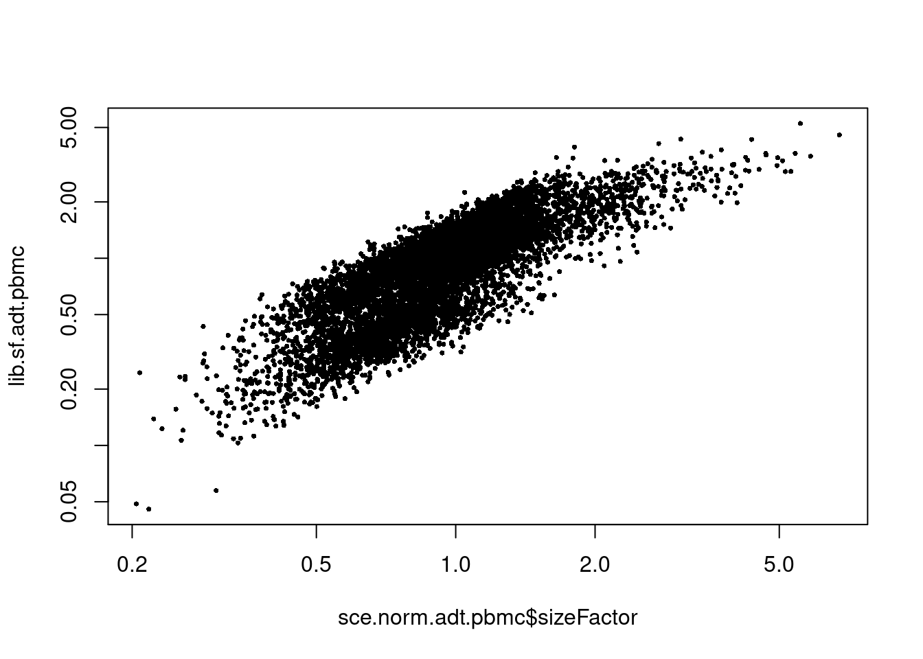
Figure 9.2: Comparison between the CLRm1 size factors and the library size-derived factors for the ADT modality of the PBMC dataset.
9.4 Feature selection and PCA
Feature selection for ADTs is generally unnecessary as it was already performed during the design of the antibody panel. The manual choice of target proteins means that all ADTs already correspond to “interesting” features. In addition, there is little scope for further filtering when the number of ADTs is low. Here, we have fewer than 20 ADTs, and even for the larger datasets, the panel will usually have less than 200 features. These are small numbers compared to our previous selections of 1000-5000 HVGs in Chapter 3.
We might consider removing the IgG controls as we know that they will not be biologically interesting. This probably won’t make much difference as the controls are unlikely to exhibit strong variation that might intefere with downstream steps. But it probably won’t hurt either, so we might as well do it:
selected.adt.pbmc <- !grepl("^IgG", rownames(sce.norm.adt.pbmc))
rowData(sce.norm.adt.pbmc)$of.interest <- selected.adt.pbmc
summary(selected.adt.pbmc)
## Mode FALSE TRUE
## logical 3 14We also perform a PCA on the ADT log-abundance matrix as described in Chapter 4. This is mostly useful for datasets with larger panels to compact the data from ~200 ADTs to 10-20 PCs. For smaller datasets, PCA is unnecessary as the number of ADTs is comparable to the typical number of PCs. Regardless, it doesn’t hurt to run a PCA in such cases - if the number of ADTs is lower than the requested number of PCs, the PC scores will simply be a rotation of the log-abundance data.
sce.pca.adt.pbmc <- runPca.se(
    sce.norm.adt.pbmc,
    features=selected.adt.pbmc,
    number=20
)
dim(reducedDim(sce.pca.adt.pbmc, "PCA"))
## [1] 7411 14If we don’t want to run a PCA, we could instead use the log-normalized abundance matrix directly in downstream analyses.
# Transpose to make it look like a reducedDim entry, so that we could plug it
# into downstream algorithms by just setting reddim.type=.
norm.adt.pbmc <- t(assay(sce.norm.adt.pbmc, "logcounts")[selected.adt.pbmc,])
reducedDim(sce.pca.adt.pbmc, "selected") <- as.matrix(norm.adt.pbmc)

# For example...
sce.kmeans.adt.pbmc <- clusterKmeans.se(sce.pca.adt.pbmc, k=10, reddim.type="selected")
summary(sce.kmeans.adt.pbmc$clusters)
## 1 2 3 4 5 6 7 8 9 10
## 916 1232 698 490 615 1249 160 549 682 8209.5 The rest of the analysis
Once we have the PCs, we can use them for clustering and visualization in the same manner as described in Chapters 5 and 6. This summarizes the heterogeneity specific to the ADT modality (Figure 9.3).
sce.nn.adt.pbmc <- runAllNeighborSteps.se(sce.pca.adt.pbmc)
table(sce.nn.adt.pbmc$clusters)
##
## 1 2 3 4 5 6 7 8 9 10 11 12 13 14 15 16
## 702 886 956 1017 208 640 570 416 409 312 292 482 135 82 160 144library(scater)
plotReducedDim(sce.nn.adt.pbmc, "TSNE", colour_by="clusters")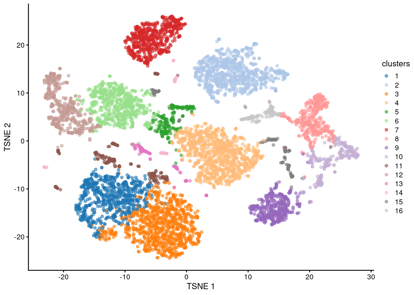
Figure 9.3: \(t\)-SNE plot generated from the log-normalized abundance of each ADT in the PBMC dataset. Each point is a cell and is colored according to its assigned cluster.
We then identify markers from the log-abundance matrix, as described in Chapter 7. For the top ADTs, we usually observe very large effect sizes due to the binary nature of surface targets. However, there are also strong composition biases in this data so some caution is required when interpreting the smaller log-fold changes.
markers.adt.pbmc <- scoreMarkers.se(sce.nn.adt.pbmc, sce.nn.adt.pbmc$clusters)
previewMarkers(markers.adt.pbmc[["1"]]) # Looking at the top marker tags for cluster 1.
## DataFrame with 10 rows and 3 columns
## mean detected lfc
## <numeric> <numeric> <numeric>
## CD14 10.47980 1.000000 4.815979
## CD4 8.93075 1.000000 1.263068
## CD15 7.23453 1.000000 0.430545
## CD56 5.42423 1.000000 0.474958
## CD45RO 7.52737 1.000000 0.355057
## IgG2a 3.28407 0.994302 0.209745
## CD16 6.25177 1.000000 0.029543
## CD25 4.45000 1.000000 0.131739
## IgG1 3.67019 0.998575 0.123389
## IgG2b 2.49592 0.961538 0.170127We can also use the ADT-derived clusters to identify marker genes from the log-expression matrix for the RNA modality. This is analogous to performing FACS to isolate cell types before differential expression analyses with bulk RNA-seq.
# Computing log-normalized expression values from the RNA counts.
sce.norm.pbmc <- normalizeRnaCounts.se(sce.qc.pbmc)

# Computing markers for RNA data but using the ADT-derived clusters!
markers.adt2rna.pbmc <- scoreMarkers.se(sce.norm.pbmc, sce.nn.adt.pbmc$clusters, extra.columns="Symbol")

# Now looking at the top marker genes for cluster 1.
previewMarkers(markers.adt2rna.pbmc[["1"]], pre.columns="Symbol")
## DataFrame with 10 rows and 4 columns
## Symbol mean detected lfc
## <character> <numeric> <numeric> <numeric>
## ENSG00000090382 LYZ 6.09956 1.000000 5.04224
## ENSG00000101439 CST3 3.88405 1.000000 3.14760
## ENSG00000011600 TYROBP 3.76942 1.000000 2.72675
## ENSG00000158869 FCER1G 3.16000 0.998575 2.36430
## ENSG00000163220 S100A9 5.93046 1.000000 4.89871
## ENSG00000085265 FCN1 3.07327 0.994302 2.55797
## ENSG00000163563 MNDA 2.71558 0.997151 2.26325
## ENSG00000163131 CTSS 3.62322 0.998575 2.64997
## ENSG00000143546 S100A8 5.24883 0.994302 4.37216
## ENSG00000025708 TYMP 2.66359 0.995726 2.12287Conversely, we could derive clusters from the RNA data and test for differential abundance of ADTs between clusters. This is most relevant when the ADTs represent some kind of functional readout (e.g., binding activity) instead of cell type identity.
9.6 Combining modalities
A more efficient use of our CITE-seq data would consider heterogeneity in both modalities simultaneously. In other words, the ADT and RNA data are combined in some manner prior to clustering and visualisations. This ensures that any unique variation in either modality will be captured in the cluster definitions. For example, if the antibody panel captures transient post-translation modifications like phosphorylation, this will not show up in the RNA data; conversely, biological processes without a surface target will not be represented in the ADT data. To demonstrate, let’s continue the analysis of the RNA modality of our PBMC dataset:
sce.var.pbmc <- chooseRnaHvgs.se(sce.norm.pbmc)
sce.pca.pbmc <- runPca.se(sce.var.pbmc, features=rowData(sce.var.pbmc)$hvg, number=20)
ncol(reducedDim(sce.pca.pbmc))
## [1] 20Possibly the simplest method to combine modalities involves literally combining the matrices of ADT- and RNA-derived PC scores. (Or if no PCA was performed for the ADTs, the log-abundance matrix can be used instead.) The combined matrix contains both sets of PCs, ensuring that heterogeneity from both modalities will be considered, e.g., when computing distances and finding neighbors. However, naively combining the two matrices is not ideal as the number of genes is typically several orders of magnitude greater than the number of ADTs. This would cause the RNA modality to dominate the variance in the combined matrix, effectively sidelining any contributions from the ADT modality.
Instead, we scale the modalities to balance their contributions to the combined matrix with the scaleByNeighbors.se() function.
For each modality, we compute the median distance from each cell to its \(k\)-nearest neighbor, which we treat as a proxy for the uninteresting variation within subpopulations.
Each matrix of PCs is then scaled according to its median distance, equalizing the magnitude of uninteresting variation across modalities.
This ensures that high baseline variation in one modality will not drown out interesting biological variation in another modality in the combined matrix.
We use the nearest neighbor distance to avoid capturing genuine biological differences between subpopulations -
otherwise, if we scaled on total variance, we would penalize the most informative modalities with the strongest heterogeneity.
# We put our ADT experiment back inside the parent object so that
# scaleByNeighbors.se can see both sets of PCs at once.
altExp(sce.pca.pbmc, "Antibody Capture") <- sce.pca.adt.pbmc

sce.combined.pbmc <- scaleByNeighbors.se(
    sce.pca.pbmc,
    main.reddims="PCA",
    altexp.reddims=c(`Antibody Capture`="PCA")
)
dim(reducedDim(sce.combined.pbmc, "combined"))
## [1] 7411 34# Scaling applied to PCs from the main experiment, i.e., the RNA.
metadata(sce.combined.pbmc)$combined$main.scaling## PCA
## 1# Scaling applied to PCs from the alternative experiment, i.e., the ADTs.
metadata(sce.combined.pbmc)$combined$altexp.scaling## $`Antibody Capture`
## PCA
## 2.195758The combined matrix of PCs is convenient as it can be used in the same functions that accept a regular matrix of PCs. Now, we can easily accommodate multiple modalities in downstream steps like clustering and visualization (Figure 9.4).
sce.nn.combined.pbmc <- runAllNeighborSteps.se(sce.combined.pbmc, reddim.type="combined")
table(sce.nn.combined.pbmc$clusters)
##
## 1 2 3 4 5 6 7 8 9 10 11 12 13 14 15 16
## 1649 730 1005 763 585 510 460 375 461 208 230 91 73 158 79 34plotReducedDim(sce.nn.combined.pbmc, "TSNE", colour_by="clusters")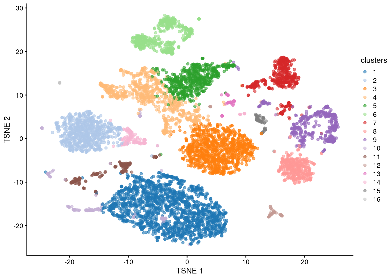
Figure 9.4: \(t\)-SnE plot of the PBMC data generated from combined ADT and RNA PCs. Each point is a cell and is colored according to the assigned cluster.
In practice, the RNA and ADT modalities are often strongly correlated when the antibody panel targets cell type-related proteins. Using a combined matrix does not offer much benefit in these cases - in fact, we would say that a well-designed panel is more than enough for cell type identification36, without any help from gene expression at all. Combining modalities may even be detrimental if one of the modalities has little biological variation, e.g., if no antibodies are bound, the ADT matrix will only be contributing noise. So, what should we do? Well, our usual advice for single-cell analysis applies, a.k.a., see if we get interesting results and try something else if we don’t.
Session information
sessionInfo()## R Under development (unstable) (2025-12-24 r89227)
## Platform: x86_64-pc-linux-gnu
## Running under: Ubuntu 22.04.5 LTS
##
## Matrix products: default
## BLAS: /home/luna/Software/R/trunk/lib/libRblas.so
## LAPACK: /home/luna/Software/R/trunk/lib/libRlapack.so; LAPACK version 3.12.1
##
## locale:
## [1] LC_CTYPE=en_US.UTF-8 LC_NUMERIC=C
## [3] LC_TIME=en_US.UTF-8 LC_COLLATE=en_US.UTF-8
## [5] LC_MONETARY=en_US.UTF-8 LC_MESSAGES=en_US.UTF-8
## [7] LC_PAPER=en_US.UTF-8 LC_NAME=C
## [9] LC_ADDRESS=C LC_TELEPHONE=C
## [11] LC_MEASUREMENT=en_US.UTF-8 LC_IDENTIFICATION=C
##
## time zone: Australia/Sydney
## tzcode source: system (glibc)
##
## attached base packages:
## [1] stats4 stats graphics grDevices utils datasets methods
## [8] base
##
## other attached packages:
## [1] scater_1.39.1 ggplot2_4.0.1
## [3] scuttle_1.21.0 scrapper_1.5.10
## [5] DropletUtils_1.31.0 SingleCellExperiment_1.33.0
## [7] SummarizedExperiment_1.41.0 Biobase_2.71.0
## [9] GenomicRanges_1.63.1 Seqinfo_1.1.0
## [11] IRanges_2.45.0 S4Vectors_0.49.0
## [13] BiocGenerics_0.57.0 generics_0.1.4
## [15] MatrixGenerics_1.23.0 matrixStats_1.5.0
## [17] DropletTestFiles_1.21.0 BiocStyle_2.39.0
##
## loaded via a namespace (and not attached):
## [1] DBI_1.2.3 gridExtra_2.3
## [3] httr2_1.2.2 rlang_1.1.7
## [5] magrittr_2.0.4 otel_0.2.0
## [7] compiler_4.6.0 RSQLite_2.4.5
## [9] DelayedMatrixStats_1.33.0 png_0.1-8
## [11] vctrs_0.6.5 pkgconfig_2.0.3
## [13] crayon_1.5.3 fastmap_1.2.0
## [15] dbplyr_2.5.1 XVector_0.51.0
## [17] labeling_0.4.3 rmarkdown_2.30
## [19] ggbeeswarm_0.7.3 purrr_1.2.1
## [21] bit_4.6.0 xfun_0.55
## [23] cachem_1.1.0 beachmat_2.27.1
## [25] jsonlite_2.0.0 blob_1.2.4
## [27] rhdf5filters_1.23.3 DelayedArray_0.37.0
## [29] Rhdf5lib_1.33.0 BiocParallel_1.45.0
## [31] irlba_2.3.5.1 parallel_4.6.0
## [33] R6_2.6.1 bslib_0.9.0
## [35] RColorBrewer_1.1-3 limma_3.67.0
## [37] jquerylib_0.1.4 Rcpp_1.1.1
## [39] bookdown_0.46 knitr_1.51
## [41] R.utils_2.13.0 Matrix_1.7-4
## [43] tidyselect_1.2.1 viridis_0.6.5
## [45] dichromat_2.0-0.1 abind_1.4-8
## [47] yaml_2.3.12 codetools_0.2-20
## [49] curl_7.0.0 lattice_0.22-7
## [51] tibble_3.3.0 S7_0.2.1
## [53] withr_3.0.2 KEGGREST_1.51.1
## [55] evaluate_1.0.5 BiocFileCache_3.1.0
## [57] ExperimentHub_3.1.0 Biostrings_2.79.4
## [59] pillar_1.11.1 BiocManager_1.30.27
## [61] filelock_1.0.3 BiocVersion_3.23.1
## [63] sparseMatrixStats_1.23.0 scales_1.4.0
## [65] glue_1.8.0 tools_4.6.0
## [67] AnnotationHub_4.1.0 BiocNeighbors_2.5.0
## [69] ScaledMatrix_1.19.0 locfit_1.5-9.12
## [71] cowplot_1.2.0 rhdf5_2.55.12
## [73] grid_4.6.0 AnnotationDbi_1.73.0
## [75] edgeR_4.9.2 beeswarm_0.4.0
## [77] BiocSingular_1.27.1 HDF5Array_1.39.0
## [79] vipor_0.4.7 rsvd_1.0.5
## [81] cli_3.6.5 rappdirs_0.3.3
## [83] viridisLite_0.4.2 S4Arrays_1.11.1
## [85] dplyr_1.1.4 gtable_0.3.6
## [87] R.methodsS3_1.8.2 sass_0.4.10
## [89] digest_0.6.39 ggrepel_0.9.6
## [91] SparseArray_1.11.10 dqrng_0.4.1
## [93] farver_2.1.2 memoise_2.0.1
## [95] htmltools_0.5.9 R.oo_1.27.1
## [97] lifecycle_1.0.5 h5mread_1.3.1
## [99] httr_1.4.7 statmod_1.5.1
## [101] bit64_4.6.0-1References
Stoeckius, M., C. Hafemeister, W. Stephenson, B. Houck-Loomis, P. K. Chattopadhyay, H. Swerdlow, R. Satija, and P. Smibert. 2017. “Simultaneous epitope and transcriptome measurement in single cells.” Nat. Methods 14 (9): 865–68.
Zheng, G. X., J. M. Terry, P. Belgrader, P. Ryvkin, Z. W. Bent, R. Wilson, S. B. Ziraldo, et al. 2017. “Massively parallel digital transcriptional profiling of single cells.” Nat. Commun. 8 (January): 14049.
In theory, we could conjugate RNA to almost anything that sticks to a cell, e.g., cholesterol, peptides, small molecule drugs… and maybe even my old friend, Malat1. Counts from these tags are analyzed in the same way as ADTs, so we’ll refer to all of them as ADTs for convenience.↩︎
At least for blood, which has been FACS’d to death.↩︎