Chapter 1 Quality Control
1.1 Motivation
In a typical scRNA-seq dataset, some of the cells will be of “low quality” for one reason or another. Perhaps the cells were damaged during dissociation, or maybe library preparation was not performed efficiently. Such low-quality libraries are problematic as they can contribute to misleading results in downstream analyses:
- They form their own distinct cluster(s), complicating interpretation of the results. Low-quality libraries generated from different cell types can cluster together based on similarities in the damage-induced expression profiles, creating artificial intermediate states or trajectories between otherwise distinct subpopulations.
- They interfere with quantification of population heterogeneity during variance estimation or principal components analysis. The first few principal components will capture differences in quality rather than biology, reducing the effectiveness of dimensionality reduction. Similarly, genes with the largest variances will be driven by differences between low- and high-quality cells.
- Many low-quality libraries have small total counts and are scaled up aggressively during normalization. This inflates the apparent expression of genes with non-zero counts in such libraries, which further contributes to inflated variances and formation of artificial clusters.
To mitigate these problems, we remove the problematic cells before proceeding with the rest of our analysis. This step is commonly referred to as quality control (QC) on the cells. (We will use “library” and “cell” interchangeably in this chapter; the distinction is more important for droplet-based data, where some libraries may not contain cells.)
1.2 Common choices of QC metrics
We use several common QC metrics to identify low-quality cells based on their expression profiles. These metrics are described below in terms of reads for Smart-seq2 data (Picelli et al. 2014), but the same definitions apply to UMI data generated by other technologies like MARS-seq and droplet-based protocols (Islam et al. 2014; Jaitin et al. 2014; Macosko et al. 2015; Klein et al. 2015).
- The library size is defined as the total sum of counts across all relevant features for each cell. Typically, the relevant features are the endogenous genes, excluding other feature types (e.g., spike-ins) or modalities (e.g., antibody-derived tags). Cells with small library sizes are likely to be of low quality as the RNA has been lost at some point during library preparation, either due to cell lysis or inefficient cDNA capture and amplification.
- The number of expressed features in each cell is defined as the number of endogenous genes with non-zero counts for that cell. Any cell with very few expressed genes is likely to be of poor quality as the diverse transcript population has not been successfully captured.
- The proportion of reads mapped to genes in the mitochondrial genome is defined relative to the library size in each cell (Islam et al. 2014; Ilicic et al. 2016). The reasoning is that, in the presence of modest damage, perforations in the cell membrane permit efflux of cytoplasmic transcript molecules but are too small to allow mitochondria to escape. This leads to a relative enrichment of mitochondrial transcripts in libraries corresponding to damaged cells. (For single-nuclei RNA-seq experiments, high proportions are also useful as they represent cells where the cytoplasm has not been successfully stripped.)
- If spike-in transcripts were used in the experiment, the proportion of reads mapped to spike-ins is defined relative to the library size plus the total spike-in count in each cell. As the same amount of spike-in RNA should have been added to each cell, any enrichment in spike-in counts indicates that endogenous RNA was lost. Thus, high spike-in proportions are indicative of poor-quality cells where endogenous RNA has been lost due to, e.g., partial cell lysis or RNA degradation during dissociation.
To demonstrate, we’ll use a small scRNA-seq dataset from A. T. L. Lun et al. (2017), which is provided with no prior QC steps. Happily enough, this dataset also contains spike-in transcripts so we can compute the spike-in proportions for each cell. These days, spike-ins are rare as they don’t work well in high-throughput scRNA-seq protocols; but this 416B dataset was generated from a good old-fashioned plate-based protocol, so if we’ve got spike-in data, we might as well use it.
library(scRNAseq)
sce.416b <- LunSpikeInData("416b")
sce.416b
## class: SingleCellExperiment
## dim: 46604 192
## metadata(0):
## assays(1): counts
## rownames(46604): ENSMUSG00000102693 ENSMUSG00000064842 ...
## ENSMUSG00000095742 CBFB-MYH11-mcherry
## rowData names(1): Length
## colnames(192): SLX-9555.N701_S502.C89V9ANXX.s_1.r_1
## SLX-9555.N701_S503.C89V9ANXX.s_1.r_1 ...
## SLX-11312.N712_S508.H5H5YBBXX.s_8.r_1
## SLX-11312.N712_S517.H5H5YBBXX.s_8.r_1
## colData names(8): cell line cell type ... spike-in addition block
## reducedDimNames(0):
## mainExpName: endogenous
## altExpNames(2): ERCC SIRV# Finding all the mitochondrial transcripts first.
location.416b <- rowRanges(sce.416b)
is.mito.416b <- which(any(seqnames(location.416b)=="MT"))
length(is.mito.416b)## [1] 37# And then computing the QC metrics from our count matrix.
library(scrapper)
sce.qc.416b <- quickRnaQc.se(
sce.416b,
subsets=list(MT=is.mito.416b),
altexp.proportions="ERCC" # omit this if no spike-ins are present.
)
summary(sce.qc.416b$sum)## Min. 1st Qu. Median Mean 3rd Qu. Max.
## 27084 856350 1111252 1165865 1328301 4398883summary(sce.qc.416b$detected)## Min. 1st Qu. Median Mean 3rd Qu. Max.
## 5609 7502 8341 8397 9208 11380summary(sce.qc.416b$subset.proportion.MT)## Min. 1st Qu. Median Mean 3rd Qu. Max.
## 0.04593 0.07294 0.08139 0.08146 0.09035 0.15617summary(sce.qc.416b$subset.proportion.ERCC)## Min. 1st Qu. Median Mean 3rd Qu. Max.
## 0.02263 0.04389 0.06161 0.06622 0.08451 0.20765A key assumption here is that these QC metrics are independent of the biological state of each cell. Poor values (e.g., low library sizes, high mitochondrial proportions) are presumed to be driven by technical factors rather than biological processes, such that the removal of the corresponding cells will not misrepresent the biology in downstream analyses. In heterogeneous datasets, this assumption is unlikely to be true:
- Some cell types have systematically less RNA content or more mitochondria (see Figure 3A of Germain, Sonrel, and Robinson (2020)). For example, CD8+ T cells increase RNA synthesis upon stimulation while hepatocyptes contain more mitochondria to power their metabolic activities.
- Even if all cell types have the same total RNA content and mitochondria counts, certain cell types may be less amenable to the scRNA-seq protocol. The obvious example is that of neurons, which are easily damaged during dissociation and often have poorer values for the QC metrics.
Major violations of this assumption could result in the loss of entire cell types prior to downstream analysis. We can check for such violations using diagnostic plots described in Section 1.4, but for now, let’s just hope for the best and proceed through this chapter.
1.3 Identifying low-quality cells
1.3.1 With adaptive thresholds
Once we have some QC metrics, we need to define thresholds with which we can separate low- and high-quality cells. With the adaptive threshold strategy, we assume that most of our dataset consists of high-quality cells. This is usually reasonable and can be experimentally verified in some situations, e.g., by visually checking that each cell is intact on a microwell plate. We then identify cells that are outliers for any of the QC metrics, based on the median absolute deviation (MAD) from the median value of each metric across all cells. By default, we consider a value to be an outlier if it is more than 3 MADs from the median in the “problematic” direction. This is loosely motivated by the fact that such a filter will retain 99% of non-outlier values that follow a normal distribution.
qc.thresh.416b <- metadata(sce.qc.416b)$qc$thresholds
qc.thresh.416b
## $sum
## [1] 434082.9
##
## $detected
## [1] 5231.468
##
## $subset.proportion
## MT ERCC
## 0.1191734 0.1454460This function computes a MAD-based outlier threshold for each metric.
- For the library sizes and number of expressed genes, a lower threshold is defined after log-transforming the metrics.
This improves the normality of right-skewed distributions to justify the 99% rationale mentioned above.
It also avoids defining a negative threshold that would be meaningless for a non-negative metric.
Note that only the MAD calculations are on the log-scale - the thresholds reported in
qc.thresh.416bare always on the original scale. - For the mitochondrial/spike-in proportions, an upper threshold is defined without any transformation of the metrics. In particular, we do not log-transform as this would inflate the MAD by converting near-zero proportions to large negative log-values.
We apply these thresholds to filter for high-quality cells where the relevant metrics are above/below their respective lower/upper thresholds:
# The 'keep' column in the colData is added by quickRnaQc.se() and indicates
# whether a cell should be kept after QC filtering.
summary(sce.qc.416b$keep)
## Mode FALSE TRUE
## logical 6 186# Subsetting our SingleCellExperiment to only retain high-quality
# cells in the downstream analysis steps.
sce.filt.416b <- sce.qc.416b[,sce.qc.416b$keep]
ncol(sce.filt.416b)## [1] 186These outlier-based thresholds adapt to both the location and spread of the distribution of values for a given metric. This enables the QC procedure to adjust to changes in sequencing depth, cDNA capture efficiency, mitochondrial content, etc. without any user intervention or prior experience. The use of the MAD also improves robustness to dependencies between the QC metrics and the underlying biology, where some cell types have extreme QC metrics due to their biology. A heterogeneous population should have higher variability in the metrics among high-quality cells, increasing the MAD and reducing the risk of inadvertently removing those cell types (at the cost of reducing power to remove actual low-quality cells).
Keep in mind that the underlying assumption of a high-quality majority may not always be appropriate. If most cells are of (unacceptably) low quality, the adaptive thresholds will fail as - by definition - they cannot remove the majority of cells. Of course, what is “acceptable” or not is rather context-dependent, e.g., small library sizes for embryonic stem cells might be problematic but the same distribution would be perfectly satisfactory for a dataset of naive T cells. In practice, this assumption is convenient as it ensures that we always retain most cells for our downstream analyses.
1.3.2 With fixed thresholds
A simpler approach to identify low-quality cells involves applying fixed thresholds to the QC metrics.
For example, we might consider cells to be low quality if they have library sizes below 100000 reads;
express fewer than 5000 genes;
have spike-in proportions above 10%;
or have mitochondrial proportions above 10%.
We can supply these numbers directly to quickRnaQc.se() to force the function to use our thresholds:
sce.fixed.416b <- quickRnaQc.se(
    sce.416b,
    subsets=list(MT=is.mito.416b),
    altexp.proportions="ERCC",
    thresholds=list(
        sum = 1e5,
        detected = 5e3,
        subsets = c(MT = 0.1, ERCC = 0.1)
    )
)

summary(sce.fixed.416b$keep)
## Mode FALSE TRUE
## logical 39 153This strategy is intuitive but requires some experience to determine appropriate thresholds for each experimental protocol and biological system. Thresholds for read count-based data are not applicable for UMI-based data, and vice versa. Differences in mitochondrial activity or total RNA content require constant adjustment of the mitochondrial and spike-in thresholds, respectively, for different biological systems. Even with the same protocol and system, the appropriate threshold can vary between runs due to fluctuations in cDNA capture efficiency and sequencing depth per cell.
1.4 Creating diagnostic plots
It’s prudent to inspect the distributions of QC metrics (Figure 1.1) to identify possible problems. In the most ideal case, we would see normal distributions that would justify the 3 MAD threshold used in outlier detection. A large proportion of cells in another mode suggests that the QC metrics might be correlated with some biological state, potentially leading to the loss of distinct cell types during filtering; or that there were inconsistencies with library preparation for a subset of cells, which is not uncommon in plate-based protocols.
library(scater)
gridExtra::grid.arrange(
    plotColData(sce.qc.416b, y="sum", colour_by="keep") +
        geom_hline(yintercept=qc.thresh.416b$sum, linetype="dashed", color="red") +
        scale_y_log10() +
        ggtitle("Total count"),
    plotColData(sce.qc.416b, y="detected", colour_by="keep") +
        geom_hline(yintercept=qc.thresh.416b$detected, linetype="dashed", color="red") +
        scale_y_log10() +
        ggtitle("Detected features"),
    plotColData(sce.qc.416b, y="subset.proportion.MT", colour_by="keep") +
        geom_hline(yintercept=qc.thresh.416b$subset.proportion["MT"], linetype="dashed", color="red") +
        ggtitle("Mito prop"),
    plotColData(sce.qc.416b, y="subset.proportion.ERCC", colour_by="keep") +
        geom_hline(yintercept=qc.thresh.416b$subset.proportion["ERCC"], linetype="dashed", color="red") +
        ggtitle("ERCC prop"),
    ncol=2
)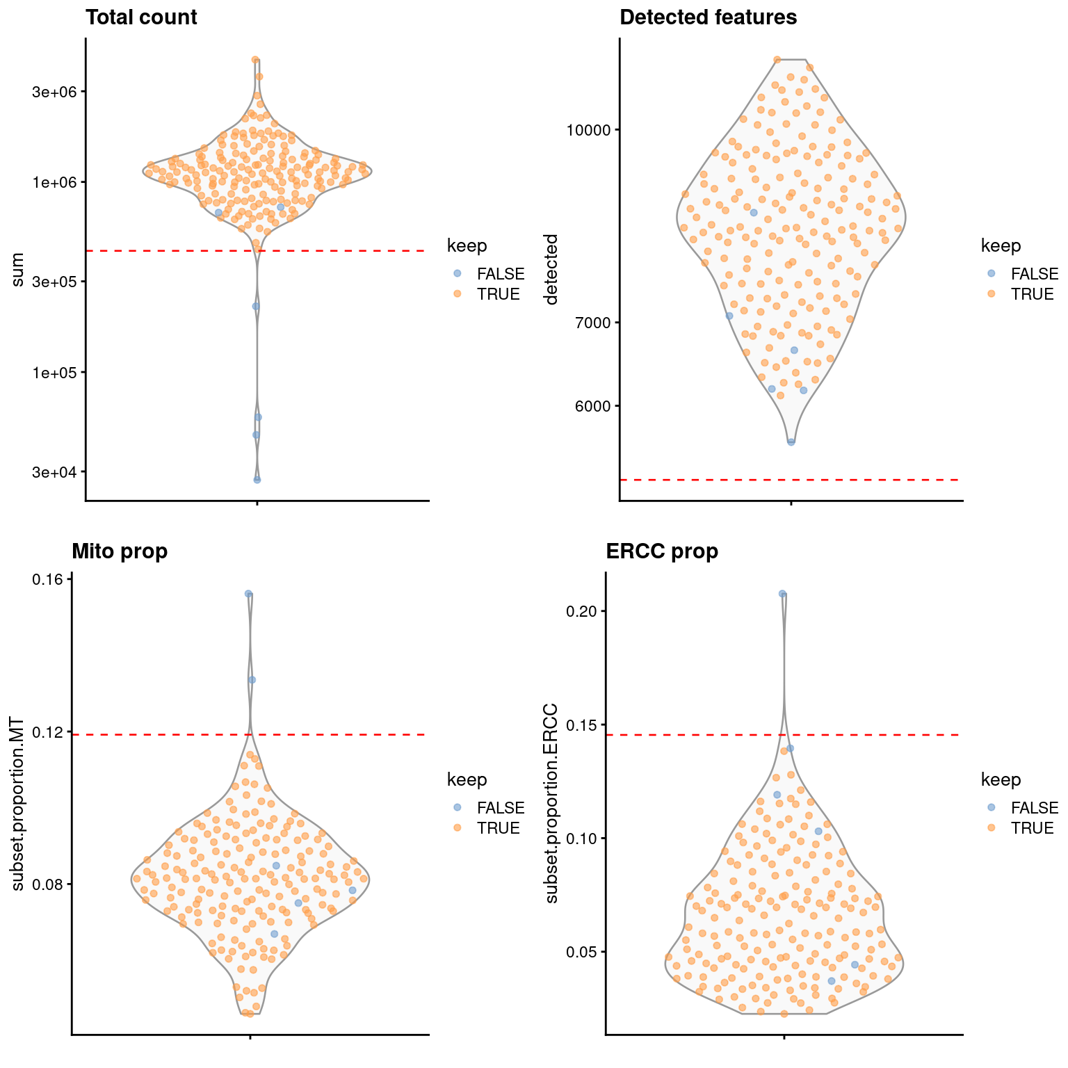
Figure 1.1: Distribution of QC metrics in the 416B dataset. Each point represents a cell and is colored according to whether it was retained after QC filtering. Dashed lines represent thresholds for each metric.
For comparison, let’s look at a different dataset with stronger biological heterogeneity (Grun et al. 2016). This dataset contains a mixture of pancreatic cell types from different donors, resulting in a more complex distribution for the metrics in Figure 1.2. We might contemplate whether the clump of discarded cells corresponds to a genuine subpopulation, though all things considered, they are probably just damaged cells and removing them is the correct choice.
library(scRNAseq)
sce.grun <- GrunPancreasData()

# This dataset doesn't include any of the mitochondrial genes, unfortunately.
# But it does contain some nice ERCC spike-ins, so let's compute those proportions.
library(scrapper)
sce.qc.grun <- quickRnaQc.se(sce.grun, subsets=list(), altexp.proportions="ERCC")
qc.thresh.grun <- metadata(sce.qc.grun)$qc$thresholds
qc.thresh.grun
## $sum
## [1] 99.01313
##
## $detected
## [1] 133.9956
##
## $subset.proportion
## ERCC
## 0.2666693summary(sce.qc.grun$keep)## Mode FALSE TRUE
## logical 437 1291library(scater)
gridExtra::grid.arrange(
plotColData(sce.qc.grun, y="sum", colour_by="keep") +
geom_hline(yintercept=qc.thresh.grun$sum, linetype="dashed", color="red") +
scale_y_log10() +
ggtitle("Total count"),
plotColData(sce.qc.grun, y="detected", colour_by="keep") +
geom_hline(yintercept=qc.thresh.grun$detected, linetype="dashed", color="red") +
scale_y_log10() +
ggtitle("Detected features"),
plotColData(sce.qc.grun, y="subset.proportion.ERCC", colour_by="keep") +
geom_hline(yintercept=qc.thresh.grun$subset.proportion["ERCC"], linetype="dashed", color="red") +
scale_y_log10() +
ggtitle("ERCC proportion"),
ncol=3
)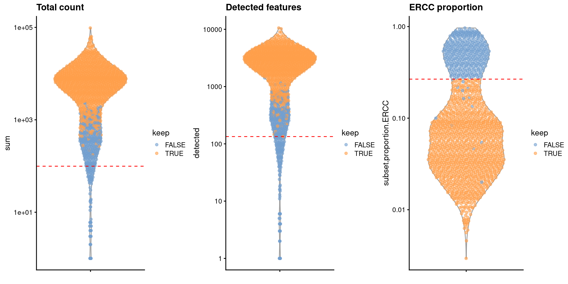
Figure 1.2: Distribution of QC metrics in the Grun dataset. Each point represents a cell and is colored according to whether it was retained after QC filtering. Dashed lines represent thresholds for each metric.
Another useful diagnostic involves comparing the proportion of mitochondrial counts against some of the other QC metrics.
- Libraries with both large total counts and large mitochondrial counts may represent high-quality cells that happen to be highly metabolically active (e.g., hepatocytes, muscle cells). A similar interpretation can be applied to libraries with high mitochondrial percentages and low spike-in percentages, if these are available.
- Low-quality cells with small mitochondrial percentages, large spike-in percentages and small library sizes are likely to be stripped nuclei, i.e., they have been so extensively damaged that they have lost all cytoplasmic content. For single-nuclei studies, the stripped nuclei become the libraries of interest while the undamaged cells are of low quality.
We demonstrate on data from a larger experiment involving the mouse brain (Zeisel et al. 2015). Figure 1.3 shows that the mitochondrial proportion is negatively correlated to the total count and positively correlated with the spike-in proportion. This is consistent with a common underlying effect of cell damage and indicates that we are not removing metabolically active, undamaged cells.
library(scRNAseq)
sce.zeisel <- ZeiselBrainData()
is.mito.zeisel <- rowData(sce.zeisel)$featureType=="mito"
summary(is.mito.zeisel)
## Mode FALSE TRUE
## logical 19972 34# This dataset also contains spike-ins, so we might as well use them.
library(scrapper)
sce.qc.zeisel <- quickRnaQc.se(sce.zeisel, subsets=list(MT=is.mito.zeisel), altexp.proportions="ERCC")
qc.thresh.zeisel <- metadata(sce.qc.zeisel)$qc$thresholds
qc.thresh.zeisel## $sum
## [1] 1928.56
##
## $detected
## [1] 845.7155
##
## $subset.proportion
## MT ERCC
## 0.2022321 0.7627049summary(sce.qc.zeisel$keep)## Mode FALSE TRUE
## logical 139 2866library(scater)
gridExtra::grid.arrange(
plotColData(sce.qc.zeisel, x="sum", y="subset.proportion.MT", colour_by="keep"),
plotColData(sce.qc.zeisel, x="subset.proportion.ERCC", y="subset.proportion.MT", colour_by="keep"),
ncol=2
)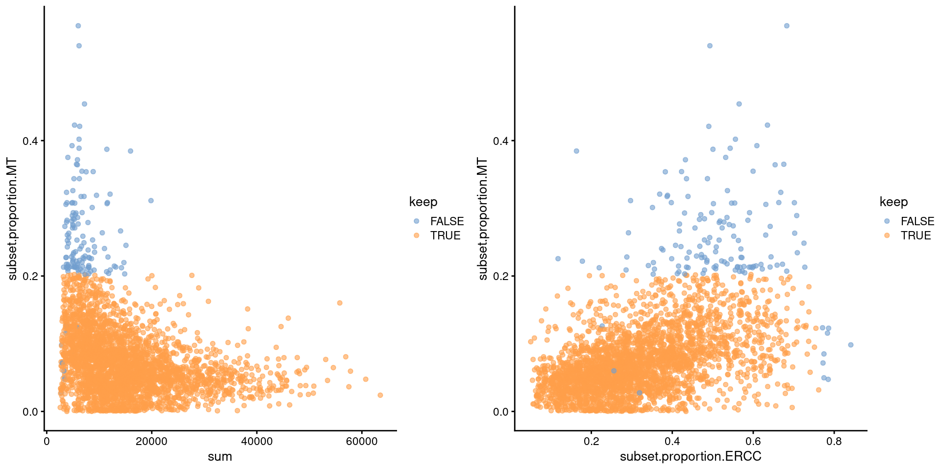
Figure 1.3: Percentage of UMIs assigned to mitochondrial transcripts in the Zeisel brain dataset, plotted against the total number of UMIs (left) or the ERCC proportions (right). Each point represents a cell and is colored according to whether it was considered high-quality.
We can also check for inappropriate removal of cell types by comparing the expression profiles of the discarded and retained cells. If the discarded pool is enriched for a certain cell type, we should observe increased expression of the corresponding marker genes. To illustrate, we’ll use the classic PBMC dataset from 10X Genomics (Zheng et al. 2017) where we perform some additional QC after cell calling. Examination of the upregulated genes in Figure 1.4 reveals PF4, PPBP and SDPR, which (spoiler alert!) indicates that there is a platelet subpopulation that was removed by our QC filter.
# Loading in raw data from the 10X output files.
library(DropletTestFiles)
raw.path.10x <- getTestFile("tenx-2.1.0-pbmc4k/1.0.0/raw.tar.gz")
dir.path.10x <- file.path(tempdir(), "pbmc4k")
untar(raw.path.10x, exdir=dir.path.10x)

library(DropletUtils)
fname.10x <- file.path(dir.path.10x, "raw_gene_bc_matrices/GRCh38")
sce.10x <- read10xCounts(fname.10x, col.names=TRUE)

# Cell calling to distinguish real cells from empty droplets. Normally this
# would be handled by the CellRanger pipeline, but older versions of CellRanger
# would already remove interesting cells with low total counts before we could
# even make any QC decisions. So for the purposes of this example, we'll handle
# cell calling ourselves using the unfiltered count data.
set.seed(100)
ed.10x <- emptyDrops(counts(sce.10x))
sce.10x <- sce.10x[,which(ed.10x$FDR <= 0.001)]
sce.10x
## class: SingleCellExperiment
## dim: 33694 4402
## metadata(1): Samples
## assays(1): counts
## rownames(33694): ENSG00000243485 ENSG00000237613 ... ENSG00000277475
## ENSG00000268674
## rowData names(2): ID Symbol
## colnames(4402): AAACCTGAGAAGGCCT-1 AAACCTGAGACAGACC-1 ...
## TTTGTCAGTTAAGACA-1 TTTGTCATCCCAAGAT-1
## colData names(2): Sample Barcode
## reducedDimNames(0):
## mainExpName: NULL
## altExpNames(0):# Applying our default QC with outlier-based thresholds.
is.mito.10x <- grepl("^MT-", rowData(sce.10x)$Symbol)
sce.qc.10x <- quickRnaQc.se(sce.10x, subsets=list(MT=is.mito.10x))
# Summing counts for the pools of retained or discarded cells.
aggregate.10x <- aggregateAcrossCells.se(
sce.10x,
list(status=ifelse(sce.qc.10x$keep, "retain", "discard"))
)
sums.10x <- assay(aggregate.10x, "sums")
colnames(sums.10x) <- aggregate.10x$factor.status
head(sums.10x)## discard retain
## ENSG00000243485 0 0
## ENSG00000237613 0 0
## ENSG00000186092 0 0
## ENSG00000238009 0 9
## ENSG00000239945 0 2
## ENSG00000239906 0 0# Computing log-fold changes between retained and discarded pools.
library(edgeR)
logged.10x <- cpm(sums.10x, log=TRUE, prior.count=2)
logFC.10x <- logged.10x[,"discard"] - logged.10x[,"retain"]
abundance.10x <- rowMeans(logged.10x)
plot(abundance.10x, logFC.10x, xlab="Average abundance", ylab="Log-FC (discarded/retained)", pch=16, cex=0.5)
platelet <- match(c("PF4", "PPBP", "SDPR"), rowData(sce.10x)$Symbol)
points(abundance.10x[platelet], logFC.10x[platelet], col="red", pch=16)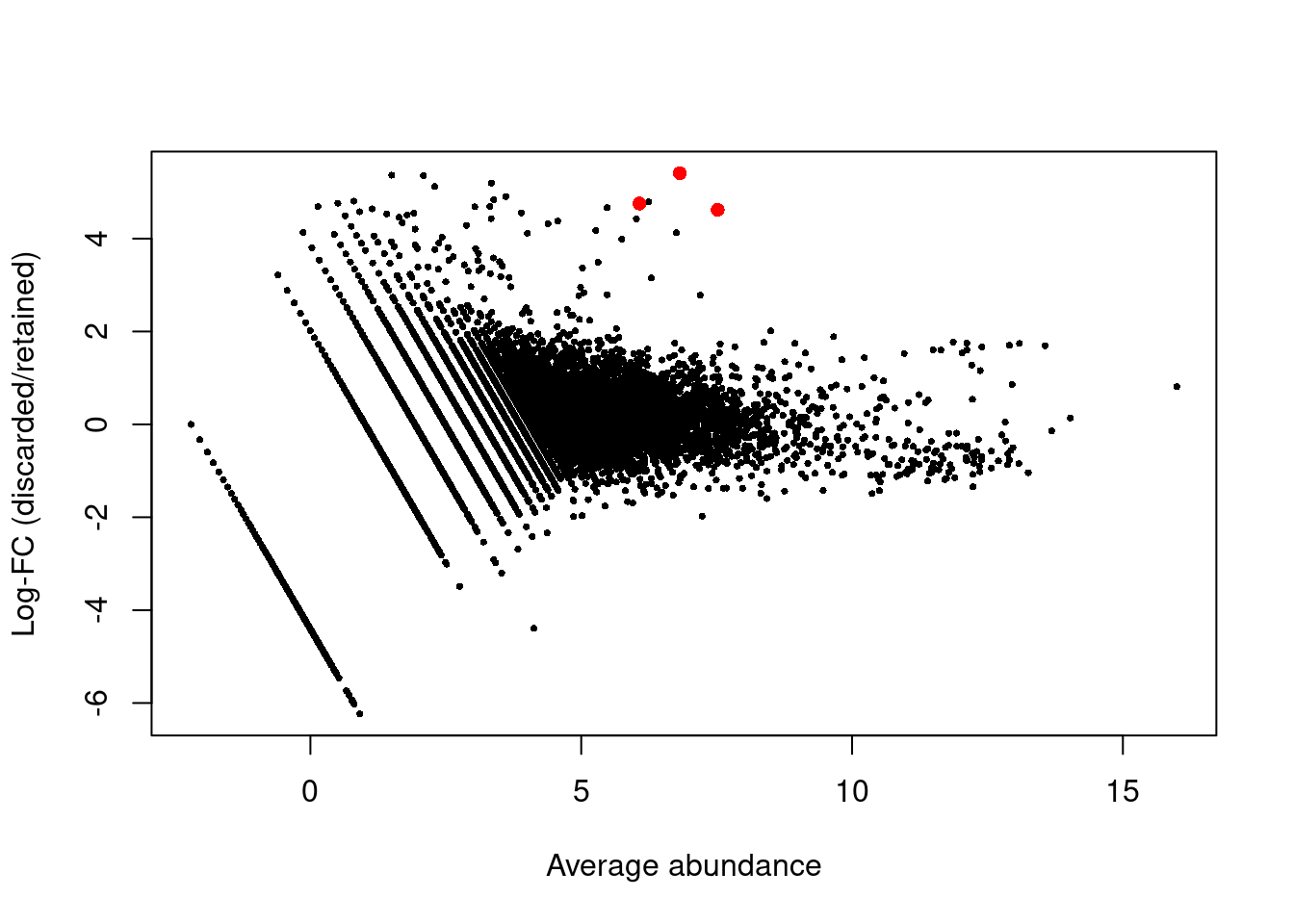
Figure 1.4: Log-fold changes between discarded and retained cells in the PBMC dataset against the average abundance. Each point represents a gene, with platelet-related genes highlighted in red.
If we suspect that cell types have been incorrectly discarded by our QC procedure, the most direct solution is to relax the QC filters.
This is easily achieved for the outlier-based thresholds by increasing num.mads= in the quickRnaQc.se() call.
Alternatively, we can disable filtering for particular metrics by setting the threshold to Inf or -Inf for upper and lower thresholds, respectively.
We might even think about skipping the filtering altogether1,
as discussed in Section 1.6.
# Effectively just filtering on the mitochondrial proportions.
relaxed.thresh.10x <- metadata(sce.qc.10x)$qc$thresholds
relaxed.thresh.10x$sum <- -Inf
relaxed.thresh.10x$detected <- -Inf
sce.relaxed.10x <- quickRnaQc.se(
    sce.10x,
    subsets=list(MT=is.mito.10x),
    thresholds=relaxed.thresh.10x
)
summary(sce.relaxed.10x$keep)
## Mode FALSE TRUE
## logical 322 40801.5 Blocking on experimental factors
More complex studies may involve multiple blocks of cells generated with different experimental parameters, e.g., sequencing depth. In such cases, it makes little sense to compute medians and MADs from a mixture distribution containing samples from multiple blocks. For example, if the sequencing coverage is lower in one block compared to the others, the median will be dragged down and the MAD will be inflated. This will reduce the suitability of the adaptive threshold for each block.
A possibly better approach is to compute an adaptive threshold separately for each block, under the assumption that most cells in each block are of high quality.
We illustrate using our 416B dataset again, which actually contains two experimental factors that we previously ignored:
the microwell plate in which each cell was processed, and whether the expression of a CBFB-MYH11 oncogene was induced by doxycycline treatment.
For the purposes of QC, we will consider each unique combination of these factors to be an experimental block,
as both have the potential to alter the QC metrics, e.g., different sequencing coverage in each run or different RNA content after treatment.
Setting block= in quickRnaQc.se() yields a separate threshold for each block (Figure 1.5),
which may be more appropriate than a common threshold across all blocks.
# Making a combined factor for easier reading.
plate.416b <- sce.416b$block # i.e., the plate of origin.
pheno.416b <- ifelse(sce.416b$phenotype == "wild type phenotype", "WT", "induced")
block.416b <- paste0(pheno.416b, "-", plate.416b)

sce.block.416b <- quickRnaQc.se(
    sce.416b,
    subsets=list(MT=is.mito.416b),
    altexp.proportions="ERCC",
    block=block.416b
)
qc.thresh.block.416b <- metadata(sce.block.416b)$qc$thresholds
qc.thresh.block.416b
## $sum
## induced-20160113 induced-20160325 WT-20160113 WT-20160325
## 461073.1 399133.7 599794.9 370316.5
##
## $detected
## induced-20160113 induced-20160325 WT-20160113 WT-20160325
## 5399.240 6519.740 7215.887 7586.402
##
## $subset.proportion
## $subset.proportion$MT
## induced-20160113 induced-20160325 WT-20160113 WT-20160325
## 0.1175679 0.1289473 0.1175331 0.1169890
##
## $subset.proportion$ERCC
## induced-20160113 induced-20160325 WT-20160113 WT-20160325
## 0.15504768 0.12718583 0.08995810 0.08105749
##
##
## $block.ids
## [1] "induced-20160113" "induced-20160325" "WT-20160113" "WT-20160325"summary(sce.block.416b$keep)## Mode FALSE TRUE
## logical 9 183library(scater)
sce.block.416b$combined.block <- block.416b
gridExtra::grid.arrange(
plotColData(sce.block.416b, y="sum", x="combined.block", colour_by="keep") +
categoricalHlinesNamed(qc.thresh.block.416b$sum, levels=NULL, linetype="dashed", color="red") +
scale_x_discrete(guide = guide_axis(angle = 45)) +
scale_y_log10() +
ggtitle("Total count"),
plotColData(sce.block.416b, y="detected", x="combined.block", colour_by="keep") +
categoricalHlinesNamed(qc.thresh.block.416b$detected, levels=NULL, linetype="dashed", color="red") +
scale_x_discrete(guide = guide_axis(angle = 45)) +
scale_y_log10() +
ggtitle("Detected features"),
plotColData(sce.block.416b, y="subset.proportion.MT", x="combined.block", colour_by="keep") +
categoricalHlinesNamed(qc.thresh.block.416b$subset.proportion$MT, levels=NULL, linetype="dashed", color="red") +
scale_x_discrete(guide = guide_axis(angle = 45)) +
ggtitle("Mito proportion"),
plotColData(sce.block.416b, y="subset.proportion.ERCC", x="combined.block", colour_by="keep") +
categoricalHlinesNamed(qc.thresh.block.416b$subset.proportion$ERCC, levels=NULL, linetype="dashed", color="red") +
scale_x_discrete(guide = guide_axis(angle = 45)) +
ggtitle("ERCC proportion"),
ncol=2
)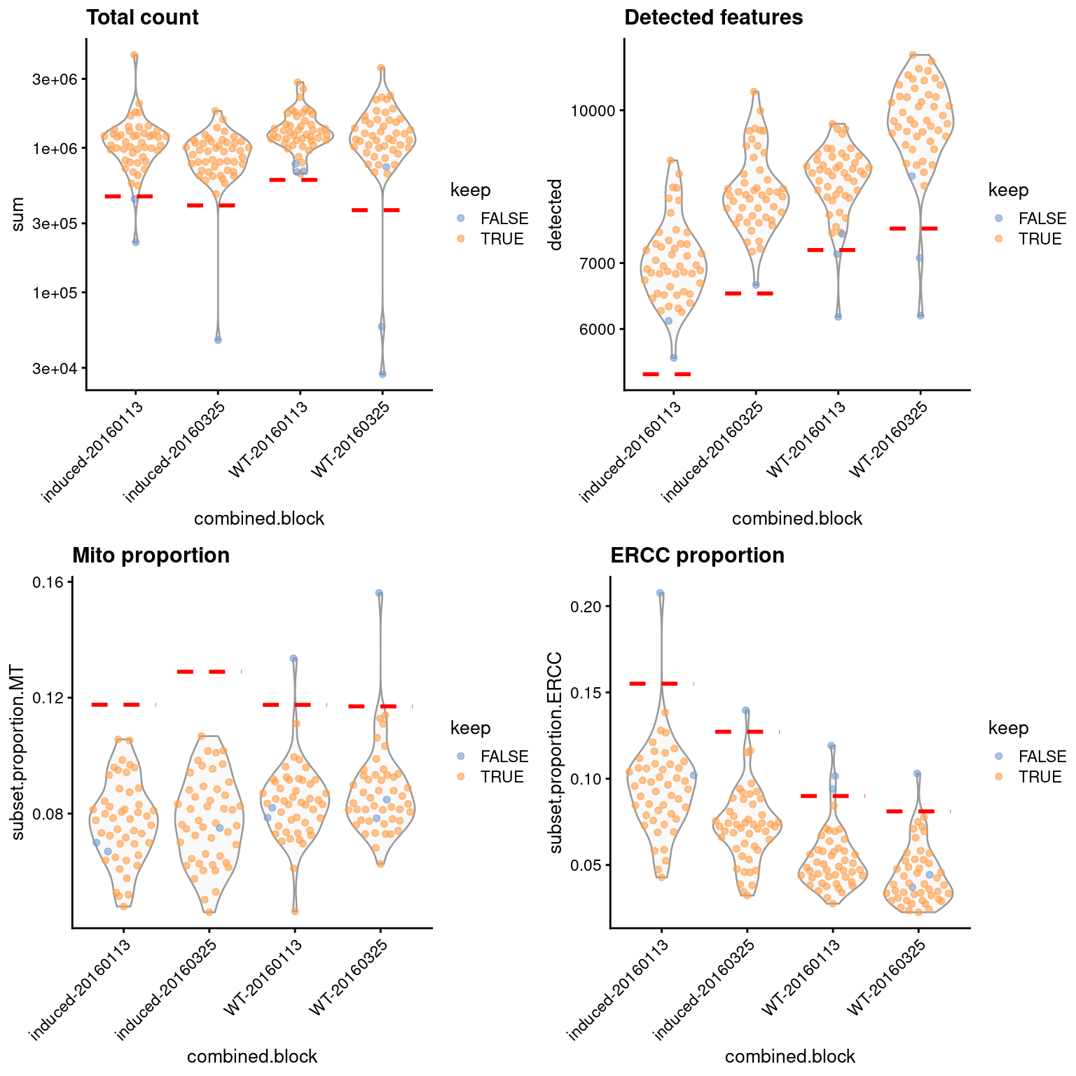
Figure 1.5: Distribution of QC metrics in the 416B dataset, separated according to each cell’s combination of experimental factors. Each point represents a cell and is colored according to whether it was retained after QC filtering. Dashed lines represent thresholds for each metric in each combination of factors.
That said, outlier detection will not be effective if a block does not contain a majority of high-quality cells. For example, some donors in the Grun et al. (2016) human pancreas dataset have higher ERCC proportions (Figure 1.6), probably corresponding to damaged cells. This inflates the median and MAD and reduces the effectiveness of the QC filtering in those blocks.
sce.block.grun <- quickRnaQc.se(
    sce.grun,
    subsets=list(),
    altexp.proportions="ERCC",
    block=sce.grun$donor
)
qc.thresh.block.grun <- metadata(sce.block.grun)$qc$thresholds
qc.thresh.block.grun
## $sum
## D10 D17 D2 D3 D7
## 1.222967 1002.354420 943.017540 3.977602 883.043512
##
## $detected
## D10 D17 D2 D3 D7
## 2.002534 815.811991 866.701785 5.936999 656.102224
##
## $subset.proportion
## $subset.proportion$ERCC
## D10 D17 D2 D3 D7
## 0.73610696 0.07599947 0.06010975 1.13105828 0.15216956
##
##
## $block.ids
## [1] "D10" "D17" "D2" "D3" "D7"summary(sce.block.grun$keep)## Mode FALSE TRUE
## logical 132 1596plotColData(sce.block.grun, x="donor", y="subset.proportion.ERCC", colour_by="keep") +
categoricalHlinesNamed(qc.thresh.block.grun$subset.proportion$ERCC, levels=NULL, linetype="dashed", color="red") +
ggtitle("ERCC prop")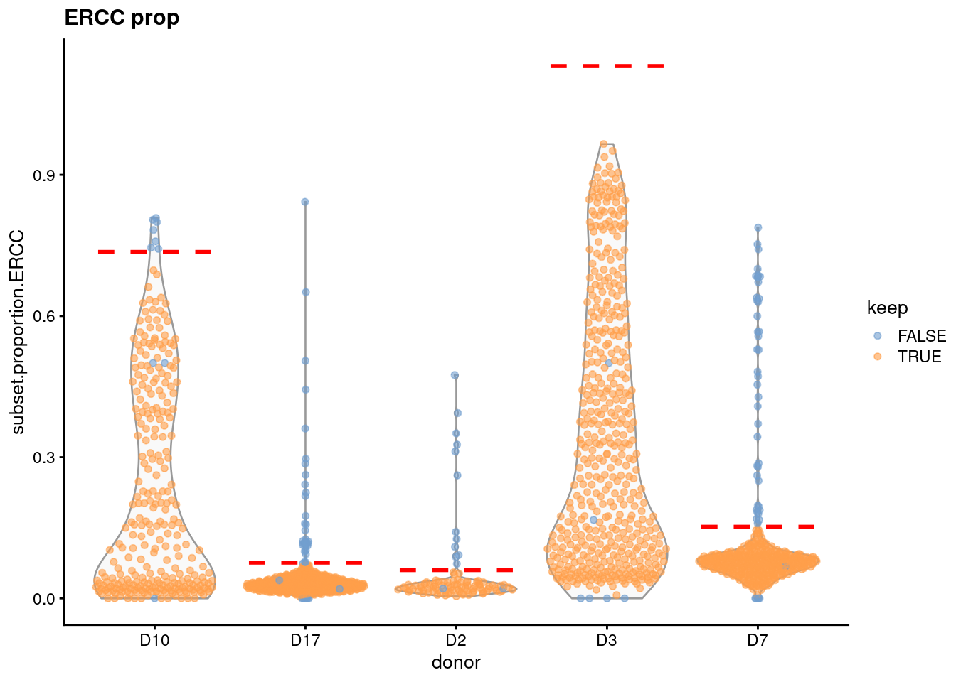
Figure 1.6: Distribution of the proportion of ERCC transcripts in each donor of the Grun pancreas dataset. Each point represents a cell and is coloured according to whether it was considered high-quality across all metrics. Dashed lines represent donor-specific thresholds.
For such problematic blocks, some manual intervention may be necessary to set an appropriate threshold. A simple solution is to just derive a threshold from the other blocks, e.g., by taking the average (Figure 1.7). This restores some semblance of QC to remove the bulk of damaged cells in the affected donors. Hopefully, those cells really are damaged and we aren’t accidentally removing a real subpopulation of small cells that are unique to those donors2.
okay.donors <- c("D17", "D2", "D7")
bad.donors <- setdiff(unique(sce.grun$donor), okay.donors)

qc.thresh.fixed.grun <- qc.thresh.block.grun
qc.thresh.fixed.grun$sum[bad.donors] <- mean(qc.thresh.block.grun$sum[okay.donors])
qc.thresh.fixed.grun$detected[bad.donors] <- mean(qc.thresh.block.grun$detected[okay.donors])
qc.thresh.fixed.grun$subset.proportion$ERCC[bad.donors] <- mean(qc.thresh.block.grun$subset.proportion$ERCC[okay.donors])

sce.fixed.grun <- quickRnaQc.se(
    sce.grun,
    subsets=list(),
    altexp.proportions="ERCC",
    block=sce.grun$donor,
    thresholds=qc.thresh.fixed.grun
)

plotColData(sce.fixed.grun, x="donor", y="subset.proportion.ERCC", colour_by="keep") +
    categoricalHlinesNamed(qc.thresh.fixed.grun$subset.proportion$ERCC, levels=NULL, linetype="dashed", color="red") +
    ggtitle("ERCC prop")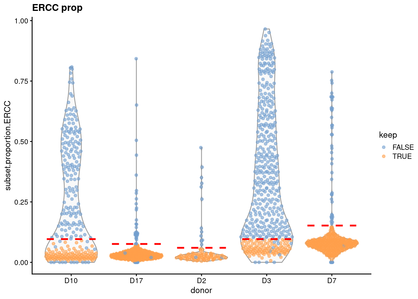
Figure 1.7: Distribution of the proportion of ERCC transcripts in each donor of the Grun pancreas dataset. Each point represents a cell and is coloured according to whether it was considered high-quality across all metrics. Dashed lines represent donor-specific thresholds, some of which are manually set for donors with a majority of low-quality cells.
1.6 Skipping quality control
If we don’t want to risk discarding real cell types, we could simply mark the low-quality cells as such and retain them in the downstream analysis.
The aim here is to allow clusters of low-quality cells to form, and then to identify and ignore such clusters during interpretation of the results.
This approach avoids discarding cell types that have poor values for the QC metrics, deferring the decision on whether a cluster of such cells represents a genuine biological state.
So, in our 416B example, we would just continue with the unfiltered sce.416b for downstream analysis instead of using sce.qc.416b.
The downside is that it shifts the burden of QC to the manual interpretation of the clusters, which is already a major bottleneck in scRNA-seq data analysis (Chapters 6 and 7). If we don’t trust the QC metrics, we would have to distinguish between genuine cell types and low-quality cells based only on the cluster-specific marker genes… but if we had good markers for low-quality cells, we would have already used them as QC metrics! In practice, this usually becomes a time-consuming process of elimination whereby the clusters of low-quality cells are identified because they don’t fit any other characterization. Additionally, retention of low-quality cells may compromise the accuracy of other steps in the analysis, as discussed in Section 1.1.
Personally, I’d suggest removing low-quality cells by default to avoid complications. This allows most of the population structure to be characterized with fewer concerns about its validity. Once the initial analysis is done, and if there are any concerns about discarded cell types, a more thorough re-analysis can be performed where the low-quality cells are only marked. This recovers cell types with low RNA content, high mitochondrial proportions, etc. that only need to be interpreted insofar as they “fill the gaps” in the initial analysis.
Session Info
sessionInfo()## R Under development (unstable) (2025-12-24 r89227)
## Platform: x86_64-pc-linux-gnu
## Running under: Ubuntu 22.04.5 LTS
##
## Matrix products: default
## BLAS: /home/luna/Software/R/trunk/lib/libRblas.so
## LAPACK: /home/luna/Software/R/trunk/lib/libRlapack.so; LAPACK version 3.12.1
##
## locale:
## [1] LC_CTYPE=en_US.UTF-8 LC_NUMERIC=C
## [3] LC_TIME=en_US.UTF-8 LC_COLLATE=en_US.UTF-8
## [5] LC_MONETARY=en_US.UTF-8 LC_MESSAGES=en_US.UTF-8
## [7] LC_PAPER=en_US.UTF-8 LC_NAME=C
## [9] LC_ADDRESS=C LC_TELEPHONE=C
## [11] LC_MEASUREMENT=en_US.UTF-8 LC_IDENTIFICATION=C
##
## time zone: Australia/Sydney
## tzcode source: system (glibc)
##
## attached base packages:
## [1] stats4 stats graphics grDevices utils datasets methods
## [8] base
##
## other attached packages:
## [1] edgeR_4.9.2 limma_3.67.0
## [3] DropletUtils_1.31.0 DropletTestFiles_1.21.0
## [5] scater_1.39.1 ggplot2_4.0.1
## [7] scuttle_1.21.0 scrapper_1.5.10
## [9] ensembldb_2.35.0 AnnotationFilter_1.35.0
## [11] GenomicFeatures_1.63.1 AnnotationDbi_1.73.0
## [13] scRNAseq_2.25.0 SingleCellExperiment_1.33.0
## [15] SummarizedExperiment_1.41.0 Biobase_2.71.0
## [17] GenomicRanges_1.63.1 Seqinfo_1.1.0
## [19] IRanges_2.45.0 S4Vectors_0.49.0
## [21] BiocGenerics_0.57.0 generics_0.1.4
## [23] MatrixGenerics_1.23.0 matrixStats_1.5.0
##
## loaded via a namespace (and not attached):
## [1] RColorBrewer_1.1-3 jsonlite_2.0.0
## [3] magrittr_2.0.4 ggbeeswarm_0.7.3
## [5] gypsum_1.7.0 farver_2.1.2
## [7] rmarkdown_2.30 BiocIO_1.21.0
## [9] vctrs_0.6.5 DelayedMatrixStats_1.33.0
## [11] memoise_2.0.1 Rsamtools_2.27.0
## [13] RCurl_1.98-1.17 htmltools_0.5.9
## [15] S4Arrays_1.11.1 AnnotationHub_4.1.0
## [17] curl_7.0.0 BiocNeighbors_2.5.0
## [19] Rhdf5lib_1.33.0 SparseArray_1.11.10
## [21] rhdf5_2.55.12 sass_0.4.10
## [23] alabaster.base_1.11.1 bslib_0.9.0
## [25] alabaster.sce_1.11.0 httr2_1.2.2
## [27] cachem_1.1.0 GenomicAlignments_1.47.0
## [29] lifecycle_1.0.5 pkgconfig_2.0.3
## [31] rsvd_1.0.5 Matrix_1.7-4
## [33] R6_2.6.1 fastmap_1.2.0
## [35] digest_0.6.39 dqrng_0.4.1
## [37] irlba_2.3.5.1 ExperimentHub_3.1.0
## [39] RSQLite_2.4.5 beachmat_2.27.1
## [41] labeling_0.4.3 filelock_1.0.3
## [43] httr_1.4.7 abind_1.4-8
## [45] compiler_4.6.0 bit64_4.6.0-1
## [47] withr_3.0.2 S7_0.2.1
## [49] BiocParallel_1.45.0 viridis_0.6.5
## [51] DBI_1.2.3 R.utils_2.13.0
## [53] HDF5Array_1.39.0 alabaster.ranges_1.11.0
## [55] alabaster.schemas_1.11.0 rappdirs_0.3.3
## [57] DelayedArray_0.37.0 rjson_0.2.23
## [59] tools_4.6.0 vipor_0.4.7
## [61] otel_0.2.0 beeswarm_0.4.0
## [63] R.oo_1.27.1 glue_1.8.0
## [65] h5mread_1.3.1 restfulr_0.0.16
## [67] rhdf5filters_1.23.3 grid_4.6.0
## [69] gtable_0.3.6 R.methodsS3_1.8.2
## [71] BiocSingular_1.27.1 ScaledMatrix_1.19.0
## [73] XVector_0.51.0 ggrepel_0.9.6
## [75] BiocVersion_3.23.1 pillar_1.11.1
## [77] dplyr_1.1.4 BiocFileCache_3.1.0
## [79] lattice_0.22-7 rtracklayer_1.71.3
## [81] bit_4.6.0 tidyselect_1.2.1
## [83] locfit_1.5-9.12 Biostrings_2.79.4
## [85] knitr_1.51 gridExtra_2.3
## [87] bookdown_0.46 ProtGenerics_1.43.0
## [89] xfun_0.55 statmod_1.5.1
## [91] UCSC.utils_1.7.1 lazyeval_0.2.2
## [93] yaml_2.3.12 evaluate_1.0.5
## [95] codetools_0.2-20 cigarillo_1.1.0
## [97] tibble_3.3.0 alabaster.matrix_1.11.0
## [99] BiocManager_1.30.27 cli_3.6.5
## [101] jquerylib_0.1.4 dichromat_2.0-0.1
## [103] Rcpp_1.1.1 GenomeInfoDb_1.47.2
## [105] dbplyr_2.5.1 png_0.1-8
## [107] XML_3.99-0.20 parallel_4.6.0
## [109] blob_1.2.4 sparseMatrixStats_1.23.0
## [111] bitops_1.0-9 viridisLite_0.4.2
## [113] alabaster.se_1.11.0 scales_1.4.0
## [115] purrr_1.2.1 crayon_1.5.3
## [117] rlang_1.1.7 cowplot_1.2.0
## [119] KEGGREST_1.51.1References
Germain, P.-L., A. Sonrel, and M. D. Robinson. 2020. “pipeComp, a general framework for the evaluation of computational pipelines, reveals performant single cell RNA-seq preprocessing tools.” Genome Biol. 21 (1): 227.
Grun, D., M. J. Muraro, J. C. Boisset, K. Wiebrands, A. Lyubimova, G. Dharmadhikari, M. van den Born, et al. 2016. “De novo prediction of stem cell identity using single-cell transcriptome data.” Cell Stem Cell 19 (2): 266–77.
Ilicic, T., J. K. Kim, A. A. Kołodziejczyk, F. O. Bagger, D. J. McCarthy, J. C. Marioni, and S. A. Teichmann. 2016. “Classification of low quality cells from single-cell RNA-seq data.” Genome Biol. 17 (1): 29.
Islam, S., A. Zeisel, S. Joost, G. La Manno, P. Zajac, M. Kasper, P. Lonnerberg, and S. Linnarsson. 2014. “Quantitative single-cell RNA-seq with unique molecular identifiers.” Nat. Methods 11 (2): 163–66.
Jaitin, D. A., E. Kenigsberg, H. Keren-Shaul, N. Elefant, F. Paul, I. Zaretsky, A. Mildner, et al. 2014. “Massively parallel single-cell RNA-seq for marker-free decomposition of tissues into cell types.” Science 343 (6172): 776–79.
Klein, A. M., L. Mazutis, I. Akartuna, N. Tallapragada, A. Veres, V. Li, L. Peshkin, D. A. Weitz, and M. W. Kirschner. 2015. “Droplet barcoding for single-cell transcriptomics applied to embryonic stem cells.” Cell 161 (5): 1187–1201.
Lun, A. T. L., F. J. Calero-Nieto, L. Haim-Vilmovsky, B. Gottgens, and J. C. Marioni. 2017. “Assessing the reliability of spike-in normalization for analyses of single-cell RNA sequencing data.” Genome Res. 27 (11): 1795–1806.
Macosko, E. Z., A. Basu, R. Satija, J. Nemesh, K. Shekhar, M. Goldman, I. Tirosh, et al. 2015. “Highly parallel genome-wide expression profiling of individual cells using nanoliter droplets.” Cell 161 (5): 1202–14.
Picelli, S., O. R. Faridani, A. K. Bjorklund, G. Winberg, S. Sagasser, and R. Sandberg. 2014. “Full-length RNA-seq from single cells using Smart-seq2.” Nat. Protoc. 9 (1): 171–81.
Zeisel, A., A. B. Munoz-Manchado, S. Codeluppi, P. Lonnerberg, G. La Manno, A. Jureus, S. Marques, et al. 2015. “Brain structure. Cell types in the mouse cortex and hippocampus revealed by single-cell RNA-seq.” Science 347 (6226): 1138–42.
Zheng, G. X., J. M. Terry, P. Belgrader, P. Ryvkin, Z. W. Bent, R. Wilson, S. B. Ziraldo, et al. 2017. “Massively parallel digital transcriptional profiling of single cells.” Nat. Commun. 8 (January): 14049.